1. Quickstart
This brief first part illustrates—without much explanation—the usage of the DX Analytics library. It models two risk factors, two derivatives instruments and values these in a portfolio context.
[1]:
import dx
import datetime as dt
import pandas as pd
from pylab import plt
plt.style.use('seaborn')
1.1. Risk Factor Models
The first step is to define a model for the risk-neutral discounting.
[2]:
r = dx.constant_short_rate('r', 0.01)
We then define a market environment containing the major parameter specifications needed,
[3]:
me_1 = dx.market_environment('me', dt.datetime(2016, 1, 1))
[4]:
me_1.add_constant('initial_value', 100.)
  # starting value of simulated processes
me_1.add_constant('volatility', 0.2)
  # volatiltiy factor
me_1.add_constant('final_date', dt.datetime(2017, 6, 30))
  # horizon for simulation
me_1.add_constant('currency', 'EUR')
  # currency of instrument
me_1.add_constant('frequency', 'W')
  # frequency for discretization
me_1.add_constant('paths', 10000)
  # number of paths
me_1.add_curve('discount_curve', r)
  # number of paths
Next, the model object for the first risk factor, based on the geometric Brownian motion (Black-Scholes-Merton (1973) model).
[5]:
gbm_1 = dx.geometric_brownian_motion('gbm_1', me_1)
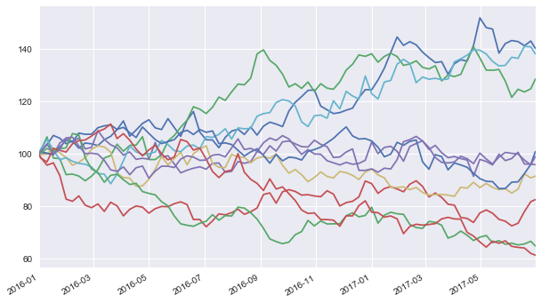
Some paths visualized.
[6]:
pdf = pd.DataFrame(gbm_1.get_instrument_values(), index=gbm_1.time_grid)
[7]:
%matplotlib inline
pdf.iloc[:, :10].plot(legend=False, figsize=(10, 6));
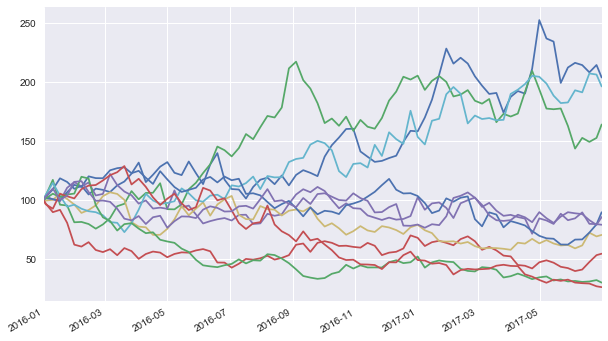
Second risk factor with higher volatility. We overwrite the respective value in the market environment.
[8]:
me_2 = dx.market_environment('me_2', me_1.pricing_date)
me_2.add_environment(me_1)  # add complete environment
me_2.add_constant('volatility', 0.5)  # overwrite value
[9]:
gbm_2 = dx.geometric_brownian_motion('gbm_2', me_2)
[10]:
pdf = pd.DataFrame(gbm_2.get_instrument_values(), index=gbm_2.time_grid)
[11]:
pdf.iloc[:, :10].plot(legend=False, figsize=(10, 6));
1.2. Valuation Models
Based on the risk factors, we can then define derivatives models for valuation. To this end, we need to add at least one (the maturity), in general two (maturity and strike), parameters to the market environments.
[12]:
me_opt = dx.market_environment('me_opt', me_1.pricing_date)
me_opt.add_environment(me_1)
me_opt.add_constant('maturity', dt.datetime(2017, 6, 30))
me_opt.add_constant('strike', 110.)
The first derivative is an American put option on the first risk factor gbm_1.
[13]:
am_put = dx.valuation_mcs_american_single(
            name='am_put',
            underlying=gbm_1,
            mar_env=me_opt,
            payoff_func='np.maximum(strike - instrument_values, 0)')
Let us calculate a Monte Carlo present value estimate and estimates for the option Greeks.
[14]:
am_put.present_value()
[14]:
15.013
[15]:
am_put.delta()
[15]:
-0.5411
[16]:
am_put.gamma()
[16]:
-0.0082
[17]:
am_put.vega()
[17]:
51.1584
[18]:
am_put.theta()
[18]:
-3.7421
[19]:
am_put.rho()
[19]:
-71.1355
The second derivative is a European call option on the second risk factor gbm_2.
[20]:
eur_call = dx.valuation_mcs_european_single(
            name='eur_call',
            underlying=gbm_2,
            mar_env=me_opt,
            payoff_func='np.maximum(maturity_value - strike, 0)')
Valuation and Greek estimation for this option.
[21]:
eur_call.present_value()
[21]:
20.641978
[22]:
eur_call.delta()
[22]:
0.8496
[23]:
eur_call.gamma()
[23]:
0.0057
[24]:
eur_call.vega()
[24]:
48.2888
[25]:
eur_call.theta()
[25]:
-8.7493
[26]:
eur_call.rho()
[26]:
54.3995
1.3. Excursion: SABR Model
To illustrate how general the approach of DX Analytics is, let us quickly analyze an option based on a SABR stochastic volatility process. In what follows herafter, the SABR model does not play a role.
We need to define different parameters obviously.
[27]:
me_3 = dx.market_environment('me_3', me_1.pricing_date)
me_3.add_environment(me_1)  # add complete environment
[28]:
# interest rate like parmeters
me_3.add_constant('initial_value', 0.05)
  # initial value
me_3.add_constant('alpha', 0.1)
  # initial variance
me_3.add_constant('beta', 0.5)
  # exponent
me_3.add_constant('rho', 0.1)
  # correlation factor
me_3.add_constant('vol_vol', 0.5)
  # volatility of volatility/variance
The model object instantiation.
[29]:
sabr = dx.sabr_stochastic_volatility('sabr', me_3)
The valuation object instantiation.
[30]:
me_opt.add_constant('strike', me_3.get_constant('initial_value'))
[31]:
sabr_call = dx.valuation_mcs_european_single(
            name='sabr_call',
            underlying=sabr,
            mar_env=me_opt,
            payoff_func='np.maximum(maturity_value - strike, 0)')
Some statistics — same syntax/API even if the model is more complex.
[32]:
sabr_call.present_value(fixed_seed=True)
[32]:
0.025849
[33]:
sabr_call.delta()
[33]:
0.8151
[34]:
sabr_call.rho()
[34]:
-0.0385
[35]:
# resetting the option strike
me_opt.add_constant('strike', 110.)
1.4. Options Portfolio
1.4.1. Modeling
In a portfolio context, we need to add information about the model class(es) to be used to the market environments of the risk factors.
[36]:
me_1.add_constant('model', 'gbm')
me_2.add_constant('model', 'gbm')
To compose a portfolio consisting of our just defined options, we need to define derivatives positions. Note that this step is independent from the risk factor model and option model definitions. We only use the market environment data and some additional information needed (e.g. payoff functions).
[37]:
put = dx.derivatives_position(
            name='put',
            quantity=2,
            underlyings=['gbm_1'],
            mar_env=me_opt,
            otype='American single',
            payoff_func='np.maximum(strike - instrument_values, 0)')
[38]:
call = dx.derivatives_position(
            name='call',
            quantity=3,
            underlyings=['gbm_2'],
            mar_env=me_opt,
            otype='European single',
            payoff_func='np.maximum(maturity_value - strike, 0)')
Let us define the relevant market by 2 Python dictionaries, the correlation between the two risk factors and a valuation environment.
[39]:
risk_factors = {'gbm_1': me_1, 'gbm_2' : me_2}
correlations = [['gbm_1', 'gbm_2', -0.4]]
positions = {'put' : put, 'call' : call}
[40]:
val_env = dx.market_environment('general', dt.datetime(2016, 1, 1))
val_env.add_constant('frequency', 'W')
val_env.add_constant('paths', 10000)
val_env.add_constant('starting_date', val_env.pricing_date)
val_env.add_constant('final_date', val_env.pricing_date)
val_env.add_curve('discount_curve', r)
These are used to define the derivatives portfolio.
[41]:
port = dx.derivatives_portfolio(
            name='portfolio',  # name
            positions=positions,  # derivatives positions
            val_env=val_env,  # valuation environment
            risk_factors=risk_factors, # relevant risk factors
            correlations=correlations, # correlation between risk factors
            parallel=False)  # parallel valuation
1.4.2. Simulation and Valuation
Now, we can get the position values for the portfolio via the get_values method.
[42]:
port.get_values()
Total
 pos_value    91.269955
dtype: float64
[42]:
| position | name | quantity | otype | risk_facts | value | currency | pos_value | |
|---|---|---|---|---|---|---|---|---|
| 0 | put | put | 2 | American single | [gbm_1] | 15.029000 | EUR | 30.058000 |
| 1 | call | call | 3 | European single | [gbm_2] | 20.403985 | EUR | 61.211955 |
Via the get_statistics methods delta and vega values are provided as well.
[43]:
port.get_statistics()
Totals
 pos_value     91.2700
pos_delta      0.5310
pos_vega     225.1372
dtype: float64
[43]:
| position | name | quantity | otype | risk_facts | value | currency | pos_value | pos_delta | pos_vega | |
|---|---|---|---|---|---|---|---|---|---|---|
| 0 | put | put | 2 | American single | [gbm_1] | 15.029 | EUR | 30.058 | -1.1802 | 87.3484 |
| 1 | call | call | 3 | European single | [gbm_2] | 20.404 | EUR | 61.212 | 1.7112 | 137.7888 |
Much more complex scenarios are possible with DX Analytics
1.4.3. Risk Reports
Having modeled the derivatives portfolio, risk reports are only two method calls away.
[44]:
deltas, benchvalue = port.get_port_risk(Greek='Delta')
gbm_2
0.8
0.9
1.0
1.1
1.2

gbm_1
0.8
0.9
1.0
1.1
1.2
[45]:
deltas
[45]:
| gbm_2_Delta | gbm_1_Delta | ||
|---|---|---|---|
| major | minor | ||
| 0.8 | factor | 80.000000 | 80.000000 |
| value | 61.767112 | 122.001955 | |
| 0.9 | factor | 90.000000 | 90.000000 |
| value | 75.421234 | 104.903955 | |
| 1.0 | factor | 100.000000 | 100.000000 |
| value | 91.269955 | 91.269955 | |
| 1.1 | factor | 110.000000 | 110.000000 |
| value | 109.161973 | 80.751955 | |
| 1.2 | factor | 120.000000 | 120.000000 |
| value | 128.739235 | 73.195955 |
[46]:
deltas.loc(axis=0)[:, 'value'] - benchvalue
[46]:
| gbm_2_Delta | gbm_1_Delta | ||
|---|---|---|---|
| major | minor | ||
| 0.8 | value | -29.502843 | 30.732 |
| 0.9 | value | -15.848721 | 13.634 |
| 1.0 | value | 0.000000 | 0.000 |
| 1.1 | value | 17.892018 | -10.518 |
| 1.2 | value | 37.469280 | -18.074 |
[47]:
vegas, benchvalue = port.get_port_risk(Greek='Vega', step=0.05)
gbm_2
0.8
0.8500000000000001
0.9000000000000001
0.9500000000000002
1.0000000000000002
1.0500000000000003
1.1000000000000003
1.1500000000000004
1.2000000000000004

gbm_1
0.8
0.8500000000000001
0.9000000000000001
0.9500000000000002
1.0000000000000002
1.0500000000000003
1.1000000000000003
1.1500000000000004
1.2000000000000004
[48]:
vegas
[48]:
| gbm_2_Vega | gbm_1_Vega | ||
|---|---|---|---|
| major | minor | ||
| 0.80 | factor | 0.400000 | 0.160000 |
| value | 77.334907 | 87.597955 | |
| 0.85 | factor | 0.430000 | 0.170000 |
| value | 80.843542 | 88.473955 | |
| 0.90 | factor | 0.450000 | 0.180000 |
| value | 84.336475 | 89.377955 | |
| 0.95 | factor | 0.480000 | 0.190000 |
| value | 87.812380 | 90.351955 | |
| 1.00 | factor | 0.500000 | 0.200000 |
| value | 91.269955 | 91.269955 | |
| 1.05 | factor | 0.530000 | 0.210000 |
| value | 94.708426 | 92.143955 | |
| 1.10 | factor | 0.550000 | 0.220000 |
| value | 98.125972 | 93.137955 | |
| 1.15 | factor | 0.580000 | 0.230000 |
| value | 101.519533 | 94.045955 | |
| 1.20 | factor | 0.600000 | 0.240000 |
| value | 104.887072 | 95.013955 |
[49]:
vegas.loc(axis=0)[:, 'value'] - benchvalue
[49]:
| gbm_2_Vega | gbm_1_Vega | ||
|---|---|---|---|
| major | minor | ||
| 0.80 | value | -13.935048 | -3.672 |
| 0.85 | value | -10.426413 | -2.796 |
| 0.90 | value | -6.933480 | -1.892 |
| 0.95 | value | -3.457575 | -0.918 |
| 1.00 | value | 0.000000 | 0.000 |
| 1.05 | value | 3.438471 | 0.874 |
| 1.10 | value | 6.856017 | 1.868 |
| 1.15 | value | 10.249578 | 2.776 |
| 1.20 | value | 13.617117 | 3.744 |
Copyright, License & Disclaimer
© Dr. Yves J. Hilpisch | The Python Quants GmbH
DX Analytics (the “dx library” or “dx package”) is licensed under the GNU Affero General Public License version 3 or later (see http://www.gnu.org/licenses/).
DX Analytics comes with no representations or warranties, to the extent permitted by applicable law.
http://tpq.io | dx@tpq.io | http://twitter.com/dyjh
Quant Platform | http://pqp.io
Python for Finance Training | http://training.tpq.io
Certificate in Computational Finance | http://compfinance.tpq.io
Derivatives Analytics with Python (Wiley Finance) | http://dawp.tpq.io
Python for Finance (2nd ed., O’Reilly) | http://py4fi.tpq.io