3. Model Classes¶

The model classes represent the fundamental building blocks to model a financial market. They are used to represent the fundamental risk factors driving uncertainty (e.g. a stock, an equity index an interest rate). The following models are available:

geometric_brownian_motion: Black-Scholes-Merton (1973) geometric Brownian motion
jump_diffusion: Merton (1976) jump diffusion
stochastic_volatility: Heston (1993) stochastic volatility model
stoch_vol_jump_diffusion: Bates (1996) stochastic volatility jump diffusion
sabr_stochastic_volatility: Hagan et al. (2002) stochastic volatility model
mean_reverting_diffusion: Vasicek (1977) short rate model
square_root_diffusion: Cox-Ingersoll-Ross (1985) square-root diffusion
square_root_jump_diffusion: square-root jump diffusion (experimental)
square_root_jump_diffusion_plus: square-root jump diffusion plus term structure (experimental)

[1]:

from dx import *
from pylab import plt
plt.style.use('seaborn')

[2]:

np.set_printoptions(precision=3)

Throughout this section we fix a constant_short_rate discounting object.

[3]:

r = constant_short_rate('r', 0.06)

3.1. geometric_brownian_motion¶

To instantiate any kind of model class, you need a market_environment object conataining a minimum set of data (depending on the specific model class).

[4]:

me = market_environment(name='me', pricing_date=dt.datetime(2015, 1, 1))

For the geometric Browniam motion class, the minimum set is as follows with regard to the constant parameter values. Here, we simply make assumptions, in practice the single values would, for example be retrieved from a data service provider like Thomson Reuters or Bloomberg. The frequency parameter is according to the pandas frequency conventions (cf. http://pandas.pydata.org/pandas-docs/stable/timeseries.html).

[5]:

me.add_constant('initial_value', 36.)
me.add_constant('volatility', 0.2)
me.add_constant('final_date', dt.datetime(2015, 12, 31))
  # time horizon for the simulation
me.add_constant('currency', 'EUR')
me.add_constant('frequency', 'M')
  # monthly frequency; paramter accorind to pandas convention
me.add_constant('paths', 1000)
  # number of paths for simulation

Every model class needs a discounting object since this defines the risk-neutral drift of the risk factor.

[6]:

me.add_curve('discount_curve', r)

The instantiation of a model class is then accomplished by providing a name as a string object and the respective market_environment object.

[7]:

gbm = geometric_brownian_motion('gbm', me)

The generate_time_grid method generates a ndarray objet of datetime objects given the specifications in the market environment. This represents the discretization of the time interval between the pricing_date and the final_date. This method does not need to be called actively.

[8]:

gbm.generate_time_grid()

[9]:

gbm.time_grid

[9]:

array([datetime.datetime(2015, 1, 1, 0, 0),
       datetime.datetime(2015, 1, 31, 0, 0),
       datetime.datetime(2015, 2, 28, 0, 0),
       datetime.datetime(2015, 3, 31, 0, 0),
       datetime.datetime(2015, 4, 30, 0, 0),
       datetime.datetime(2015, 5, 31, 0, 0),
       datetime.datetime(2015, 6, 30, 0, 0),
       datetime.datetime(2015, 7, 31, 0, 0),
       datetime.datetime(2015, 8, 31, 0, 0),
       datetime.datetime(2015, 9, 30, 0, 0),
       datetime.datetime(2015, 10, 31, 0, 0),
       datetime.datetime(2015, 11, 30, 0, 0),
       datetime.datetime(2015, 12, 31, 0, 0)], dtype=object)

The simulation itself is initiated by a call of the method get_instrument_values. It returns an ndarray object containing the simulated paths for the risk factor.

[10]:

paths = gbm.get_instrument_values()

[11]:

paths[:, :2]

[11]:

array([[36.   , 36.   ],
       [35.819, 39.084],
       [35.857, 36.918],
       [35.808, 40.226],
       [36.941, 39.883],
       [35.171, 43.389],
       [38.559, 44.775],
       [37.54 , 43.593],
       [37.977, 39.925],
       [36.249, 38.091],
       [37.665, 40.338],
       [36.593, 39.91 ],
       [36.716, 41.727]])

These can, for instance, be visualized easily. First some plotting parameter specifications we want to use throughout.

[12]:

%matplotlib inline
colormap='RdYlBu_r'
lw=1.25
figsize=(10, 6)
legend=False
no_paths=10

For easy plotting, we put the data with the time_grid information into a pandas DataFrame object.

[13]:

pdf = pd.DataFrame(paths, index=gbm.time_grid)

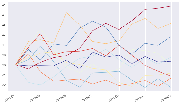
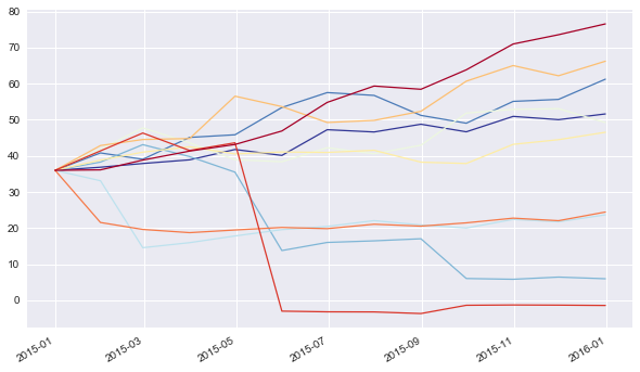
The following visualizes the first 10 paths of the simulation.

[14]:

pdf[pdf.columns[:no_paths]].plot(colormap=colormap, lw=lw,
                           figsize=figsize, legend=legend);

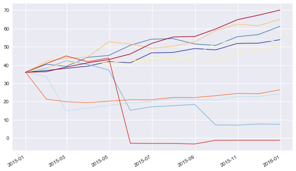
3.2. jump_diffusion¶

The next model is the jump diffusion model from Merton (1976) adding a log-normally distributed jump component to the geometric Brownian motion. Three more parameter values are needed:

[15]:

me.add_constant('lambda', 0.7)
  # probability for a jump p.a.
me.add_constant('mu', -0.8)
  # expected relative jump size
me.add_constant('delta', 0.1)
  # standard deviation of relative jump

The instantiation of the model class and usage then is the same as before.

[16]:

jd = jump_diffusion('jd', me)

[17]:

paths = jd.get_instrument_values()

[18]:

pdf = pd.DataFrame(paths, index=jd.time_grid)

[19]:

pdf[pdf.columns[:no_paths]].plot(colormap=colormap, lw=lw,
                           figsize=figsize, legend=legend);

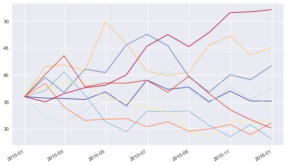
3.3. stochastic_volatility¶

Another important financial model is the stochastic volatility model according to Heston (1993). Compared to the geometric Brownian motion, this model class need four more parameter values.

[20]:

me.add_constant('rho', -.5)
  # correlation between risk factor process (eg index)
  # and variance process
me.add_constant('kappa', 2.5)
  # mean reversion factor
me.add_constant('theta', 0.1)
  # long-term variance level
me.add_constant('vol_vol', 0.1)
  # volatility factor for variance process

Again, the instantiation and usage of this model class are essentially the same.

[21]:

sv = stochastic_volatility('sv', me)

The following visualizes 10 simulated paths for the risk factor process.

[22]:

paths = sv.get_instrument_values()

[23]:

pdf = pd.DataFrame(paths, index=sv.time_grid)

[24]:

# index level paths
pdf[pdf.columns[:no_paths]].plot(colormap=colormap, lw=lw,
                           figsize=figsize, legend=legend);

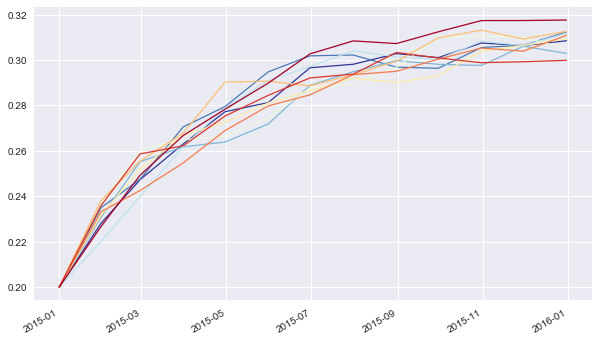
This model class has a second set of simulated paths, namely for the variance process.

[25]:

vols = sv.get_volatility_values()

[26]:

pdf = pd.DataFrame(vols, index=sv.time_grid)

[27]:

# volatility paths
pdf[pdf.columns[:no_paths]].plot(colormap=colormap, lw=lw,
                           figsize=figsize, legend=legend);

3.4. stoch_vol_jump_diffusion¶

The next model class, i.e. stoch_vol_jump_diffusion, combines stochastic volatility with a jump diffusion according to Bates (1996). Our market environment object me contains already all parameters needed for the instantiation of this model.

[28]:

svjd = stoch_vol_jump_diffusion('svjd', me)

As with the stochastic_volatility class, this class generates simulated paths for both the risk factor and variance process.

[29]:

paths = svjd.get_instrument_values()

[30]:

pdf = pd.DataFrame(paths, index=svjd.time_grid)

[31]:

# index level paths
pdf[pdf.columns[:no_paths]].plot(colormap=colormap, lw=lw,
                           figsize=figsize, legend=legend);

[32]:

vols = svjd.get_volatility_values()

[33]:

pdf = pd.DataFrame(vols, index=svjd.time_grid)

[34]:

# volatility paths
pdf[pdf.columns[:no_paths]].plot(colormap=colormap, lw=lw,
                           figsize=figsize, legend=legend);

3.5. sabr_stochastic_volatility¶

The sabr_stochastic_volatility model is based on the Hagan et al. (2002) paper. It needs the following parameters:

[35]:

# short rate like parameters
me.add_constant('initial_value', 0.5)
  # starting value (eg inital short rate)
me.add_constant('alpha', 0.04)
  # initial variance
me.add_constant('beta', 0.5)
  # exponent
me.add_constant('rho', 0.1)
  # correlation factor
me.add_constant('vol_vol', 0.5)
  # volatility of volatility/variance

[36]:

sabr = sabr_stochastic_volatility('sabr', me)

[37]:

paths = sabr.get_instrument_values()

[38]:

pdf = pd.DataFrame(paths, index=sabr.time_grid)

[39]:

pdf[pdf.columns[:no_paths]].plot(colormap=colormap, lw=lw,
                           figsize=figsize, legend=legend);

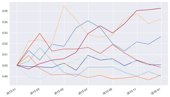
[40]:

vols = sabr.get_volatility_values()

[41]:

pdf = pd.DataFrame(vols, index=sabr.time_grid)

[42]:

pdf[pdf.columns[:no_paths]].plot(colormap=colormap, lw=lw,
                           figsize=figsize, legend=legend);

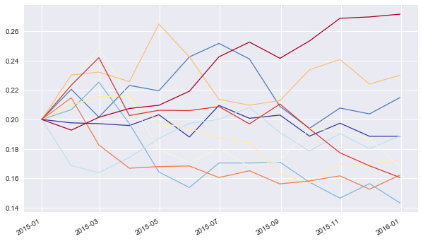
3.6. mean_reverting_diffusion¶

The mean_reverting_diffusion model class is based on the Vasicek (1977) short rate model. It is suited to model mean-reverting quantities, like short rates, volatilities, etc. The model needs the following set of parameters:

[43]:

# short rate like parameters
me.add_constant('initial_value', 0.05)
  # starting value (eg inital short rate)
me.add_constant('volatility', 0.05)
  # volatility factor
me.add_constant('kappa', 2.5)
  # mean reversion factor
me.add_constant('theta', 0.01)
  # long-term mean

[44]:

mrd = mean_reverting_diffusion('mrd', me)

[45]:

paths = mrd.get_instrument_values()

[46]:

pdf_1 = pd.DataFrame(paths, index=mrd.time_grid)

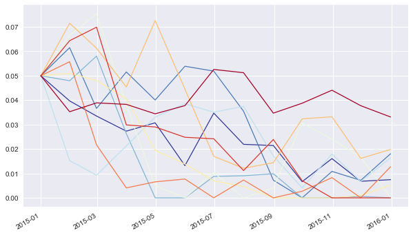
Simulated paths can go negative which might be undesireable, e.g. when modeling volatility processes.

[47]:

pdf_1[pdf_1.columns[:no_paths]].plot(colormap=colormap, lw=lw,
                           figsize=figsize, legend=legend);

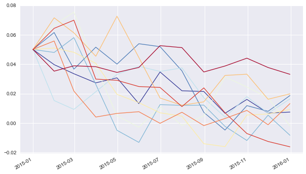
Using a full trunctation discretization scheme ensures positive paths.

[48]:

mrd = mean_reverting_diffusion('mrd', me, truncation=True)
paths = mrd.get_instrument_values()
pdf_1 = pd.DataFrame(paths, index=mrd.time_grid)

[49]:

pdf_1[pdf_1.columns[:no_paths]].plot(colormap=colormap, lw=lw,
                           figsize=figsize, legend=legend);

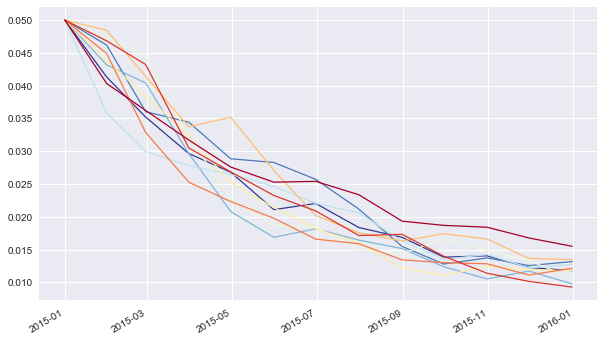
3.7. square_root_diffusion¶

The square_root_diffusion model class is based on the square-root diffusion according to Cox-Ingersoll-Ross (1985). This class is often used to model stochastic short rates or a volatility process (eg like the VSTOXX volatility index). The model needs the same parameters as the mean_reverting_diffusion.

As before, the handling of the model class is the same, making it easy to simulate paths given the parameter specifications and visualize them.

[50]:

srd = square_root_diffusion('srd', me)

[51]:

paths = srd.get_instrument_values()

[52]:

pdf_2 = pd.DataFrame(paths, index=srd.time_grid)

[53]:

pdf_2[pdf_2.columns[:no_paths]].plot(colormap=colormap, lw=lw,
                           figsize=figsize, legend=legend);

Let us compare the simulated paths — based on the same parameters — for the mean_reverting_diffusion and the square_root_diffusion in a single chart. The paths from the mean_reverting_diffusion object are much more volatile.

[54]:

ax = pdf_1[pdf_1.columns[:no_paths]].plot(style='b-.', lw=lw,
                           figsize=figsize, legend=legend);
pdf_2[pdf_1.columns[:no_paths]].plot(style='r--', lw=lw,
                           figsize=figsize, legend=legend, ax=ax);

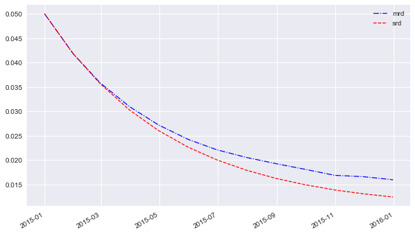
However, the mean values do not differ that much since both share the same long-term mean level. Mean reversion is faster with the square_root_diffusion model.

[55]:

ax = pdf_1.mean(axis=1).plot(style='b-.', lw=lw,
                    figsize=figsize, label='mrd', legend=True);
pdf_2.mean(axis=1).plot(style='r--', lw=lw,
                    figsize=figsize, label='srd', legend=True);

3.8. square_root_jump_diffusion¶

Experimental Status

Building on the square-root diffusion, there is a square-root jump diffusion adding a log-normally distributed jump component. The following parmeters might be for a volatility index, for example. In this case, the major risk might be a large positive jump in the index. The following model parameters are needed:

[56]:

# volatility index like parameters
me.add_constant('initial_value', 25.)
  # starting values
me.add_constant('kappa', 2.)
  # mean-reversion factor
me.add_constant('theta', 20.)
  # long-term mean
me.add_constant('volatility', 1.)
  # volatility of diffusion
me.add_constant('lambda', 0.3)
  # probability for jump p.a.
me.add_constant('mu', 0.4)
  # expected jump size
me.add_constant('delta', 0.2)
  # standard deviation of jump

Once the square_root_jump_diffusion class is instantiated, the handling of the resulting object is the same as with the other model classes.

[57]:

srjd = square_root_jump_diffusion('srjd', me)

[58]:

paths = srjd.get_instrument_values()

[59]:

pdf = pd.DataFrame(paths, index=srjd.time_grid)

[60]:

pdf[pdf.columns[:no_paths]].plot(colormap=colormap, lw=lw,
                           figsize=figsize, legend=legend);

[61]:

paths[-1].mean()

[61]:

21.93069902310944

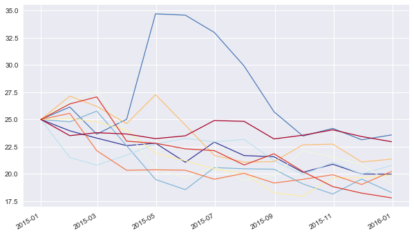
3.9. square_root_jump_diffusion_plus¶

Experimental Status

This model class further enhances the square_root_jump_diffusion class by adding a deterministic shift approach according to Brigo-Mercurio (2001) to account for a market given term structure (e.g. in volatility, interest rates). Let us define a simple term structure as follows:

[62]:

term_structure = np.array([(dt.datetime(2015, 1, 1), 25.),
                  (dt.datetime(2015, 3, 31), 24.),
                  (dt.datetime(2015, 6, 30), 27.),
                  (dt.datetime(2015, 9, 30), 28.),
                  (dt.datetime(2015, 12, 31), 30.)])

[63]:

me.add_curve('term_structure', term_structure)

[64]:

srjdp = square_root_jump_diffusion_plus('srjdp', me)

The method generate_shift_base calibrates the square-root diffusion to the given term structure (varying the parameters kappa, theta and volatility).

[65]:

srjdp.generate_shift_base((2.0, 20., 0.1))

Optimization terminated successfully.
         Current function value: 1.117824
         Iterations: 229
         Function evaluations: 431

The results are shift_base values, i.e. the difference between the model and market implied foward rates.

[66]:

srjdp.shift_base
  # difference between market and model
  # forward rates after calibration

[66]:

array([[datetime.datetime(2015, 1, 1, 0, 0), 0.0],
       [datetime.datetime(2015, 3, 31, 0, 0), -2.139861715691705],
       [datetime.datetime(2015, 6, 30, 0, 0), -0.19434592701965414],
       [datetime.datetime(2015, 9, 30, 0, 0), -0.157275574314653],
       [datetime.datetime(2015, 12, 31, 0, 0), 0.9734498133023948]],
      dtype=object)

The method update_shift_values then calculates deterministic shift values for the relevant time grid by interpolation of the shift_base values.

[67]:

srjdp.update_shift_values()

[68]:

srjdp.shift_values
  # shift values to apply to simulation scheme
  # given the shift base values

[68]:

array([[datetime.datetime(2015, 1, 1, 0, 0), 0.0],
       [datetime.datetime(2015, 1, 31, 0, 0), -0.7213017019185525],
       [datetime.datetime(2015, 2, 28, 0, 0), -1.3945166237092015],
       [datetime.datetime(2015, 3, 31, 0, 0), -2.139861715691705],
       [datetime.datetime(2015, 4, 30, 0, 0), -1.4984828842613584],
       [datetime.datetime(2015, 5, 31, 0, 0), -0.8357247584500006],
       [datetime.datetime(2015, 6, 30, 0, 0), -0.19434592701965414],
       [datetime.datetime(2015, 7, 31, 0, 0), -0.18185482991253418],
       [datetime.datetime(2015, 8, 31, 0, 0), -0.16936373280541422],
       [datetime.datetime(2015, 9, 30, 0, 0), -0.157275574314653],
       [datetime.datetime(2015, 10, 31, 0, 0), 0.22372971933891742],
       [datetime.datetime(2015, 11, 30, 0, 0), 0.5924445196488244],
       [datetime.datetime(2015, 12, 31, 0, 0), 0.9734498133023948]],
      dtype=object)

When simulating the process, the model forward rates …

[69]:

srjdp.update_forward_rates()
srjdp.forward_rates
  # model forward rates resulting from parameters

[69]:

array([[datetime.datetime(2015, 1, 1, 0, 0), 25.0],
       [datetime.datetime(2015, 1, 31, 0, 0), 22.65694757330202],
       [datetime.datetime(2015, 2, 28, 0, 0), 20.70076039334564],
       [datetime.datetime(2015, 3, 31, 0, 0), 18.797095034394516],
       [datetime.datetime(2015, 4, 30, 0, 0), 17.206256506214984],
       [datetime.datetime(2015, 5, 31, 0, 0), 15.80206686456627],
       [datetime.datetime(2015, 6, 30, 0, 0), 14.651607085467674],
       [datetime.datetime(2015, 7, 31, 0, 0), 13.652189090303105],
       [datetime.datetime(2015, 8, 31, 0, 0), 12.819382165050907],
       [datetime.datetime(2015, 9, 30, 0, 0), 12.14905682889466],
       [datetime.datetime(2015, 10, 31, 0, 0), 11.575039304260786],
       [datetime.datetime(2015, 11, 30, 0, 0), 11.116201461381866],
       [datetime.datetime(2015, 12, 31, 0, 0), 10.725486593397667]],
      dtype=object)

… are then shifted by the shift_values to better match the term structure.

[70]:

srjdp.forward_rates[:, 1] + srjdp.shift_values[:, 1]
  # shifted foward rates

[70]:

array([25.0, 21.935645871383468, 19.30624376963644, 16.65723331870281,
       15.707773621953626, 14.966342106116269, 14.45726115844802,
       13.47033426039057, 12.650018432245494, 11.991781254580006,
       11.798769023599704, 11.70864598103069, 11.698936406700062],
      dtype=object)

The simulated paths then are including the deterministic shift.

[71]:

paths = srjdp.get_instrument_values()

[72]:

pdf = pd.DataFrame(paths, index=srjdp.time_grid)

[73]:

pdf[pdf.columns[:no_paths]].plot(colormap=colormap, lw=lw,
                           figsize=figsize, legend=legend);

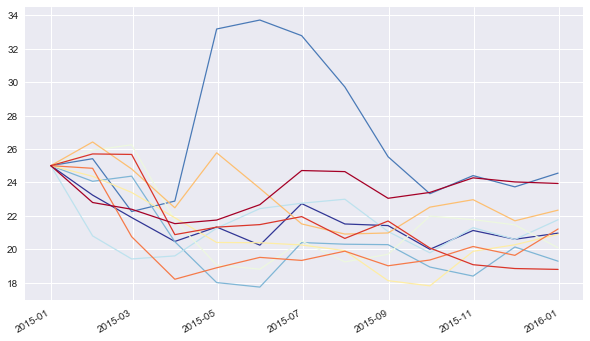
The effect might not be immediately visible in the paths plot, however, the mean of the simulated values in this case is higher by about 1 point compared to the square_root_jump_diffusion simulation without deterministic shift.

[74]:

paths[-1].mean()

[74]:

22.904148836411835

Copyright, License & Disclaimer

DX Analytics (the “dx library” or “dx package”) is licensed under the GNU Affero General Public License version 3 or later (see http://www.gnu.org/licenses/).

DX Analytics comes with no representations or warranties, to the extent permitted by applicable law.

http://tpq.io | dx@tpq.io | http://twitter.com/dyjh

Quant Platform | http://pqp.io

Python for Finance Training | http://training.tpq.io

Certificate in Computational Finance | http://compfinance.tpq.io

Derivatives Analytics with Python (Wiley Finance) | http://dawp.tpq.io

Python for Finance (2nd ed., O’Reilly) | http://py4fi.tpq.io