4. Single-Risk Derivatives Valuation
This part introduces into the modeling and valuation of derivatives instruments (contingent claims) based on a single risk factor (e.g. a stock price, stock index level or interest rate). It also shows how to model and value portfolios composed of such instruments.
[1]:
from dx import *
from pylab import plt
plt.style.use('seaborn')
The following single risk factor valuation classes are available:
valuation_mcs_european_singlefor derivatives with European exercisevaluation_mcs_american_singlefor derivatives with American/Bermudan exercise
4.1. Modeling the Risk Factor
Before moving on to the valuation classes, we need to model an instantiate an underlying risk factor, in this case a geometric_brownian_motion object. Background information is provided in the respective part of the documentation about model classes.
[2]:
r = constant_short_rate('r', 0.06)
[3]:
me = market_environment('me', dt.datetime(2015, 1, 1))
[4]:
me.add_constant('initial_value', 36.)
me.add_constant('volatility', 0.2)
me.add_constant('final_date', dt.datetime(2015, 12, 31))
me.add_constant('currency', 'EUR')
me.add_constant('frequency', 'W')
me.add_constant('paths', 25000)
[5]:
me.add_curve('discount_curve', r)
[6]:
gbm = geometric_brownian_motion('gbm', me)
4.2. valuation_mcs_european_single
The first instrument we value is a European call option written on the single relevant risk factor as embodied by the gbm model object. To this end, we add a maturity date to the market environment and a strike price.
[7]:
me.add_constant('maturity', dt.datetime(2015, 12, 31))
me.add_constant('strike', 40.)
To instantiate a the valuation_mcs_european_single class, the following information/data is to be provided:
- name as a
stringobject - instance of a model class
- market environment
- payoff of the instrument a
stringobject and containing “regular” Python/NumPy code
[8]:
call_eur = valuation_mcs_european_single(
                name='call_eur',
                underlying=gbm,
                mar_env=me,
                payoff_func='np.maximum(maturity_value - strike, 0)')
In this case, the payoff is that of a regular, plain vanilla European call option. If \(T\) is the maturity date, \(S_T\) the value of the relevant risk factor at that date and \(K\) the strike price, the payoff \(h_T\) at maturity of such an option is given by
maturity_value represents the value vector of the risk factor at maturity. Any other “sensible” payoff definition is possible. For instance, the following works as well:
[9]:
payoff = 'np.maximum(np.minimum(maturity_value) * 2 - 50, 0)'
Other standardized payoff elemenets include mean_value, max_value and min_value representing maturity value vectors with the pathwise means, maxima and minima. Using these payoff elements allows the easy definition of options with Asian features.
Having instantiated the valuation class, the present_value method returns the present value Monte Carlo estimator for the call option.
[10]:
call_eur.present_value()
[10]:
2.172619
Similarly, the delta and vega methods return the delta and the vega of the option, estimated numerically by a forward difference scheme and Monte Carlo simulation.
[11]:
call_eur.delta()
[11]:
0.4491
[12]:
call_eur.vega()
[12]:
14.1882
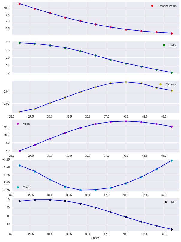
This approach allows to work with such a valuation object similar to an analytical valuation formula like the one of Black-Scholes-Merton (1973). For example, you can estimate and plot present values, deltas, gammas, vegas, thetas and rhos for a range of different initial values of the risk factor.
[13]:
%%time
k_list = np.arange(26., 46.1, 2)
pv = []; de = []; ve = []; th = []; rh = []; ga = []
for k in k_list:
    call_eur.update(strike=k)
    pv.append(call_eur.present_value())
    de.append(call_eur.delta(0.5))
    ve.append(call_eur.vega(0.2))
    th.append(call_eur.theta())
    rh.append(call_eur.rho())
    ga.append(call_eur.gamma())
CPU times: user 6.64 s, sys: 954 ms, total: 7.59 s
Wall time: 7.66 s
[14]:
%matplotlib inline
There is a little plot helper function available to plot these statistics conveniently.
[15]:
plot_option_stats_full(k_list, pv, de, ga, ve, th, rh)
4.3. valuation_mcs_american_single
The modeling and valuation of derivatives with American/Bermudan exercise is almost completely the same as in the more simple case of European exercise.
[16]:
me.add_constant('initial_value', 36.)
  # reset initial_value
[17]:
put_ame = valuation_mcs_american_single(
                name='put_eur',
                underlying=gbm,
                mar_env=me,
                payoff_func='np.maximum(strike - instrument_values, 0)')
The only difference to consider here is that for American options where exercise can take place at any time before maturity, the inner value of the option (payoff of immediate exercise) is relevant over the whole set of dates. Therefore, maturity_value needs to be replaced by instrument_values in the definition of the payoff function.
[18]:
put_ame.present_value()
[18]:
4.452
Since DX Analytics relies on Monte Carlo simulation and other numerical methods, the calculation of the delta and vega of such an option is identical to the European exercise case.
[19]:
put_ame.delta()
[19]:
-0.6655
[20]:
put_ame.vega()
[20]:
10.3122
[21]:
%%time
k_list = np.arange(26., 46.1, 2.)
pv = []; de = []; ve = []
for k in k_list:
    put_ame.update(strike=k)
    pv.append(put_ame.present_value())
    de.append(put_ame.delta(.5))
    ve.append(put_ame.vega(0.2))
CPU times: user 15.5 s, sys: 957 ms, total: 16.5 s
Wall time: 16.1 s
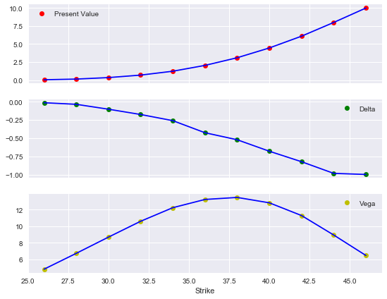
[22]:
plot_option_stats(k_list, pv, de, ve)
4.4. Portfolio Valuation
In general, market players (asset managers, investment banks, hedge funds, insurance companies, etc.) have to value not only single derivatvies instruments but rather portfolios composed of several derivatives instruments. A consistent derivatives portfolio valuation is particularly important when there are multiple derivatives written on the same risk factor and/or correlations between different risk factors.
These are the classes availble for a consistent portfolio valuation:
derivatives_positionto model a portfolio positionderivatives_portfolioto model a derivatives portfolio
4.4.1. derivatives_position
We work with the market_environment object from before and add information about the risk factor model we are using.
[23]:
me.add_constant('model', 'gbm')
A derivatives position consists of “data only” and not instantiated model or valuation objects. The necessary model and valuation objects are instantiated during the portfolio valuation.
[24]:
put = derivatives_position(
                name='put',  # name of position
                quantity=1,  # number of instruments
                underlyings=['gbm'],  # relevant risk factors
                mar_env=me,  # market environment
                otype='American single',  # the option type
                payoff_func='np.maximum(40. - instrument_values, 0)')
                    # the payoff funtion
The method get_info prints an overview of the all relevant information stored for the respective derivatives_position object.
[25]:
put.get_info()
NAME
put

QUANTITY
1

UNDERLYINGS
['gbm']

MARKET ENVIRONMENT

**Constants**
initial_value 36.0
volatility 0.2
final_date 2015-12-31 00:00:00
currency EUR
frequency W
paths 25000
maturity 2015-12-31 00:00:00
strike 40.0
model gbm

**Lists**

**Curves**
discount_curve <dx.frame.constant_short_rate object at 0x106799978>

OPTION TYPE
American single

PAYOFF FUNCTION
np.maximum(40. - instrument_values, 0)
4.4.2. derivatives_portfolio
The derivatives_portfolio class implements the core portfolio valuation tasks. This sub-section illustrates to cases, one with uncorrelated underlyings and another one with correlated underlyings
4.4.2.2. Correlated Underlyings
The second example case is exactly the same but now with a highly positive correlation between the two relevant risk factors. Correlations are to be provided as a list of list objects using the risk factor model names to reference them.
[37]:
correlations = [['gbm', 'jd', 0.9]]
Except from now passing this new object, the application and usage remains the same.
[38]:
port = derivatives_portfolio(
            name='portfolio',
            positions=positions,
            val_env=val_env,
            risk_factors=risk_factors,
            correlations=correlations,
            fixed_seed=True,
            parallel=False)
[39]:
port.get_statistics()
Totals
 pos_value    35.1350
pos_delta     1.6345
pos_vega     21.8606
dtype: float64
[39]:
| position | name | quantity | otype | risk_facts | value | currency | pos_value | pos_delta | pos_vega | |
|---|---|---|---|---|---|---|---|---|---|---|
| 0 | put | put | 1 | American single | [gbm] | 4.433 | EUR | 4.433 | -0.6548 | 10.8335 |
| 1 | call_jump | call_jump | 3 | European single | [jd] | 10.234 | EUR | 30.702 | 2.2893 | 11.0271 |
The Cholesky matrix has been added to the valuation environment (which gets passed to the risk factor model objects).
[40]:
port.val_env.lists['cholesky_matrix']
[40]:
array([[1.        , 0.        ],
       [0.9       , 0.43588989]])
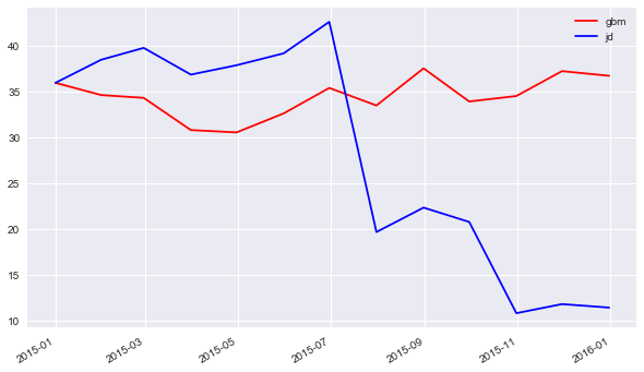
Let us pick two specific simulated paths, one for each risk factor, and let us visualize these.
[41]:
path_no = 0
paths1 = port.underlying_objects['gbm'].get_instrument_values()[:, path_no]
paths2 = port.underlying_objects['jd'].get_instrument_values()[:, path_no]
The plot illustrates that the two paths are indeed highly positively correlated. However, in this case a large jump occurs for the jump_diffusion object.
[42]:
plt.figure(figsize=(10, 6))
plt.plot(port.time_grid, paths1, 'r', label='gbm')
plt.plot(port.time_grid, paths2, 'b', label='jd')
plt.gcf().autofmt_xdate()
plt.legend(loc=0); plt.grid(True)
# highly correlated underlyings
# -- with a large jump for one risk factor
Copyright, License & Disclaimer
© Dr. Yves J. Hilpisch | The Python Quants GmbH
DX Analytics (the “dx library” or “dx package”) is licensed under the GNU Affero General Public License version 3 or later (see http://www.gnu.org/licenses/).
DX Analytics comes with no representations or warranties, to the extent permitted by applicable law.
http://tpq.io | dx@tpq.io | http://twitter.com/dyjh
Quant Platform | http://pqp.io
Python for Finance Training | http://training.tpq.io
Certificate in Computational Finance | http://compfinance.tpq.io
Derivatives Analytics with Python (Wiley Finance) | http://dawp.tpq.io
Python for Finance (2nd ed., O’Reilly) | http://py4fi.tpq.io