10. Implied Volatilities and Model Calibration
This setion of the documentation illustrates how to calculate implied volatilities and how to calibrate a model to VSTOXX volatility index call option quotes. The example implements the calibration for a total of one month worth of data.
[1]:
from dx import *
import numpy as np
import pandas as pd
from pylab import plt
plt.style.use('seaborn')
10.1. VSTOXX Futures & Options Data
We start by loading VSTOXX data from a pandas HDFStore into DataFrame objects (source: Eurex, cf. http://www.eurexchange.com/advanced-services/).
[2]:
h5 = pd.HDFStore('./data/vstoxx_march_2014.h5', 'r')
vstoxx_index = h5['vstoxx_index']
vstoxx_futures = h5['vstoxx_futures']
vstoxx_options = h5['vstoxx_options']
h5.close()
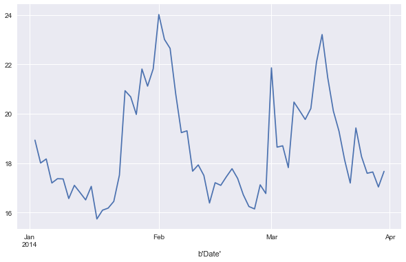
VSTOXX index for the first quarter of 2014.
[3]:
%matplotlib inline
vstoxx_index['V2TX'].plot(figsize=(10, 6))
[3]:
<matplotlib.axes._subplots.AxesSubplot at 0x115520978>
The VSTOXX futures data (8 futures maturities/quotes per day).
[4]:
vstoxx_futures.info()
<class 'pandas.core.frame.DataFrame'>
Int64Index: 504 entries, 0 to 503
Data columns (total 5 columns):
DATE         504 non-null datetime64[ns]
EXP_YEAR     504 non-null int64
EXP_MONTH    504 non-null int64
PRICE        504 non-null float64
MATURITY     504 non-null datetime64[ns]
dtypes: datetime64[ns](2), float64(1), int64(2)
memory usage: 23.6 KB
[5]:
vstoxx_futures.tail()
[5]:
| DATE | EXP_YEAR | EXP_MONTH | PRICE | MATURITY | |
|---|---|---|---|---|---|
| 499 | 2014-03-31 | 2014 | 7 | 20.40 | 2014-07-18 |
| 500 | 2014-03-31 | 2014 | 8 | 20.70 | 2014-08-15 |
| 501 | 2014-03-31 | 2014 | 9 | 20.95 | 2014-09-19 |
| 502 | 2014-03-31 | 2014 | 10 | 21.05 | 2014-10-17 |
| 503 | 2014-03-31 | 2014 | 11 | 21.25 | 2014-11-21 |
The VSTOXX options data. This data set is quite large due to the large number of European put and call options on the VSTOXX.
[6]:
vstoxx_options.info()
<class 'pandas.core.frame.DataFrame'>
Int64Index: 46960 entries, 0 to 46959
Data columns (total 7 columns):
DATE         46960 non-null datetime64[ns]
EXP_YEAR     46960 non-null int64
EXP_MONTH    46960 non-null int64
TYPE         46960 non-null object
STRIKE       46960 non-null float64
PRICE        46960 non-null float64
MATURITY     46960 non-null datetime64[ns]
dtypes: datetime64[ns](2), float64(2), int64(2), object(1)
memory usage: 2.9+ MB
[7]:
vstoxx_options.tail()
[7]:
| DATE | EXP_YEAR | EXP_MONTH | TYPE | STRIKE | PRICE | MATURITY | |
|---|---|---|---|---|---|---|---|
| 46955 | 2014-03-31 | 2014 | 11 | P | 85.0 | 63.65 | 2014-11-21 |
| 46956 | 2014-03-31 | 2014 | 11 | P | 90.0 | 68.65 | 2014-11-21 |
| 46957 | 2014-03-31 | 2014 | 11 | P | 95.0 | 73.65 | 2014-11-21 |
| 46958 | 2014-03-31 | 2014 | 11 | P | 100.0 | 78.65 | 2014-11-21 |
| 46959 | 2014-03-31 | 2014 | 11 | P | 105.0 | 83.65 | 2014-11-21 |
As a helper function we need a function to calculate all relevant third Fridays for all relevant maturity months of the data sets.
[8]:
import datetime as dt
import calendar

def third_friday(date):
    day = 21 - (calendar.weekday(date.year, date.month, 1) + 2) % 7
    return dt.datetime(date.year, date.month, day)
[9]:
third_fridays = {}
for month in set(vstoxx_futures['EXP_MONTH']):
    third_fridays[month] = third_friday(dt.datetime(2014, month, 1))
[10]:
third_fridays
[10]:
{1: datetime.datetime(2014, 1, 17, 0, 0),
 2: datetime.datetime(2014, 2, 21, 0, 0),
 3: datetime.datetime(2014, 3, 21, 0, 0),
 4: datetime.datetime(2014, 4, 18, 0, 0),
 5: datetime.datetime(2014, 5, 16, 0, 0),
 6: datetime.datetime(2014, 6, 20, 0, 0),
 7: datetime.datetime(2014, 7, 18, 0, 0),
 8: datetime.datetime(2014, 8, 15, 0, 0),
 9: datetime.datetime(2014, 9, 19, 0, 0),
 10: datetime.datetime(2014, 10, 17, 0, 0),
 11: datetime.datetime(2014, 11, 21, 0, 0)}
10.2. Implied Volatilities from Market Quotes
Often calibration efforts are undertaken to replicate the market implied volatilities or the so-called volatility surface as good as possible. With DX Analytics and the BSM_european_option class, you can efficiently calculate (i.e. numerically estimate) implied volatilities. For the example, we use the VSTOXX futures and call options data from 31. March 2014.
Some definitions, the pre-selection of option data and the pre-definition of the market environment needed.
[11]:
V0 = 17.6639  # VSTOXX level on 31.03.2014
futures_data = vstoxx_futures[vstoxx_futures.DATE == '2014/3/31'].copy()
options_data = vstoxx_options[(vstoxx_options.DATE == '2014/3/31')
                              & (vstoxx_options.TYPE == 'C')].copy()
me = market_environment('me', dt.datetime(2014, 3, 31))
me.add_constant('initial_value', 17.6639)  # index on 31.03.2014
me.add_constant('volatility', 2.0)  # for initialization
me.add_curve('discount_curve', constant_short_rate('r', 0.01))  # assumption
options_data['IMP_VOL'] = 0.0  # initialization new iv column
The following loop now calculates the implied volatilities for all those options whose strike lies within the defined tolerance level.
[12]:
%%time
tol = 0.3  # tolerance level for moneyness
for option in options_data.index:
    # iterating over all option quotes
    forward = futures_data[futures_data['MATURITY'] == \
                options_data.loc[option]['MATURITY']]['PRICE'].values
                # picking the right futures value
    if (forward * (1 - tol) < options_data.loc[option]['STRIKE']
                             < forward * (1 + tol)):
        # only for options with moneyness within tolerance
        call = options_data.loc[option]
        me.add_constant('strike', call['STRIKE'])
        me.add_constant('maturity', call['MATURITY'])
        call_option = BSM_european_option('call', me)
        options_data.loc[option, 'IMP_VOL'] = \
            call_option.imp_vol(call['PRICE'], 'call', volatility_est=0.6)
CPU times: user 691 ms, sys: 6.05 ms, total: 698 ms
Wall time: 695 ms
A selection of the results.
[13]:
options_data[60:70]
[13]:
| DATE | EXP_YEAR | EXP_MONTH | TYPE | STRIKE | PRICE | MATURITY | IMP_VOL | |
|---|---|---|---|---|---|---|---|---|
| 46230 | 2014-03-31 | 2014 | 5 | C | 12.0 | 7.55 | 2014-05-16 | 0.000000 |
| 46231 | 2014-03-31 | 2014 | 5 | C | 13.0 | 6.55 | 2014-05-16 | 0.000000 |
| 46232 | 2014-03-31 | 2014 | 5 | C | 14.0 | 5.55 | 2014-05-16 | 1.541568 |
| 46233 | 2014-03-31 | 2014 | 5 | C | 15.0 | 4.55 | 2014-05-16 | 1.321803 |
| 46234 | 2014-03-31 | 2014 | 5 | C | 16.0 | 3.65 | 2014-05-16 | 1.153001 |
| 46235 | 2014-03-31 | 2014 | 5 | C | 17.0 | 2.90 | 2014-05-16 | 1.042549 |
| 46236 | 2014-03-31 | 2014 | 5 | C | 18.0 | 2.35 | 2014-05-16 | 0.997178 |
| 46237 | 2014-03-31 | 2014 | 5 | C | 19.0 | 1.90 | 2014-05-16 | 0.969301 |
| 46238 | 2014-03-31 | 2014 | 5 | C | 20.0 | 1.55 | 2014-05-16 | 0.958777 |
| 46239 | 2014-03-31 | 2014 | 5 | C | 21.0 | 1.30 | 2014-05-16 | 0.968430 |
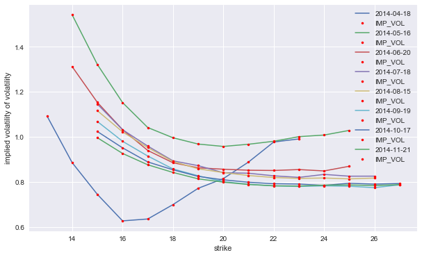
And the complete results visualized.
[14]:
import matplotlib.pyplot as plt
%matplotlib inline
plot_data = options_data[options_data.IMP_VOL > 0]
plt.figure(figsize=(10, 6))
for maturity in sorted(set(options_data['MATURITY'])):
    data = plot_data.isin({'MATURITY': [maturity,]})
    data = plot_data[plot_data.MATURITY == maturity]
      # select data for this maturity
    plt.plot(data['STRIKE'], data['IMP_VOL'],
             label=maturity.date(), lw=1.5)
    plt.plot(data['STRIKE'], data['IMP_VOL'], 'r.')
plt.xlabel('strike')
plt.ylabel('implied volatility of volatility')
plt.legend()
plt.show()
10.3. Market Modeling
This sub-section now implements the model calibration based on selected options data. In particular, we choose, for a given pricing date, the following options data:
- for a single maturity only
- call options only
- for a certain moneyness of the options
10.3.1. Relevant Market Data
The following following returns the relevant market data per calibration date:
[15]:
tol = 0.2
def get_option_selection(pricing_date, maturity, tol=tol):
    ''' Function selects relevant options data. '''
    forward = vstoxx_futures[(vstoxx_futures.DATE == pricing_date)
                & (vstoxx_futures.MATURITY == maturity)]['PRICE'].values[0]
    option_selection = \
        vstoxx_options[(vstoxx_options.DATE == pricing_date)
                     & (vstoxx_options.MATURITY == maturity)
                     & (vstoxx_options.TYPE == 'C')
                     & (vstoxx_options.STRIKE > (1 - tol) * forward)
                     & (vstoxx_options.STRIKE < (1 + tol) * forward)]
    return option_selection, forward
10.3.2. Options Modeling
Given the options and their respective quotes to which to calibrate the model, the function get_option_models returns the DX Analytics option models for all relevant options. As risk factor model we use the square_root_diffusion class.
[16]:
def get_option_models(pricing_date, maturity, option_selection):
    ''' Models and returns traded options for given option_selection object. '''
    me_vstoxx = market_environment('me_vstoxx', pricing_date)
    initial_value = vstoxx_index['V2TX'][pricing_date]
    me_vstoxx.add_constant('initial_value', initial_value)
    me_vstoxx.add_constant('final_date', maturity)
    me_vstoxx.add_constant('currency', 'EUR')
    me_vstoxx.add_constant('frequency', 'W')
    me_vstoxx.add_constant('paths', 10000)
    csr = constant_short_rate('csr', 0.01)
      # somewhat arbitrarily chosen here
    me_vstoxx.add_curve('discount_curve', csr)

    # parameters to be calibrated later
    me_vstoxx.add_constant('kappa', 1.0)
    me_vstoxx.add_constant('theta', 1.2 * initial_value)
    me_vstoxx.add_constant('volatility', 1.0)

    vstoxx_model = square_root_diffusion('vstoxx_model', me_vstoxx)
      # square-root diffusion for volatility modeling
      # mean-reverting, positive process

    # option parameters and payoff
    me_vstoxx.add_constant('maturity', maturity)
    payoff_func = 'np.maximum(maturity_value - strike, 0)'

    option_models = {}
    for option in option_selection.index:
        strike = option_selection['STRIKE'].ix[option]
        me_vstoxx.add_constant('strike', strike)
        option_models[option] = \
                            valuation_mcs_european_single(
                                    'eur_call_%d' % strike,
                                    vstoxx_model,
                                    me_vstoxx,
                                    payoff_func)
    return vstoxx_model, option_models
The function calculate_model_values estimates and returns model value estimates for all relevant options given a parameter set for the square_root_diffusion risk factor model.
[17]:
def calculate_model_values(p0):
    ''' Returns all relevant option values.

    Parameters
    ===========
    p0 : tuple/list
        tuple of kappa, theta, volatility

    Returns
    =======
    model_values : dict
        dictionary with model values
    '''
    kappa, theta, volatility = p0
    vstoxx_model.update(kappa=kappa,
                        theta=theta,
                        volatility=volatility)
    model_values = {}
    for option in option_models:
       model_values[option] = \
         option_models[option].present_value(fixed_seed=True)
    return model_values
10.4. Calibration Functions
10.4.1. Mean-Squared Error Calculation
The calibration of the pricing model is based on the minimization of the mean-squared error (MSE) of the model values vs. the market quotes. The MSE calculation is implemented by the function mean_squared_error which also penalizes economically implausible parameter values.
[18]:
i = 0
def mean_squared_error(p0):
    ''' Returns the mean-squared error given
    the model and market values.

    Parameters
    ===========
    p0 : tuple/list
        tuple of kappa, theta, volatility

    Returns
    =======
    MSE : float
        mean-squared error
    '''
    if p0[0] < 0 or p0[1] < 5. or p0[2] < 0 or p0[2] > 10.:
        return 100
    global i, option_selection, vstoxx_model, option_models, first, last
    pd = dt.datetime.strftime(
            option_selection['DATE'].iloc[0].to_pydatetime(),
            '%d-%b-%Y')
    mat = dt.datetime.strftime(
            option_selection['MATURITY'].iloc[0].to_pydatetime(),
            '%d-%b-%Y')
    model_values = calculate_model_values(p0)
    option_diffs = {}
    for option in model_values:
        option_diffs[option] = (model_values[option]
                              - option_selection['PRICE'].loc[option])
    MSE = np.sum(np.array(list(option_diffs.values())) ** 2) / len(option_diffs)
    if i % 150 == 0:
        # output every 0th and 100th iteration
        if i == 0:
            print('%12s %13s %4s  %6s  %6s  %6s  --> %6s' % \
                 ('pricing_date', 'maturity_date', 'i', 'kappa',
                  'theta', 'vola', 'MSE'))
        print('%12s %13s %4d  %6.3f  %6.3f  %6.3f  --> %6.3f' % \
                (pd, mat, i, p0[0], p0[1], p0[2], MSE))
    i += 1
    return MSE
10.4.2. Implementing the Calibration Procedure
The function get_parameter_series calibrates the model to the market data for every date contained in the pricing_date_list object for all maturities contained in the maturity_list object.
[19]:
import scipy.optimize as spo
def get_parameter_series(pricing_date_list, maturity_list):
    global i, option_selection, vstoxx_model, option_models, first, last
    # collects optimization results for later use (eg. visualization)
    parameters = pd.DataFrame()
    for maturity in maturity_list:
        first = True
        for pricing_date in pricing_date_list:
            option_selection, forward = \
                    get_option_selection(pricing_date, maturity)
            vstoxx_model, option_models = \
                    get_option_models(pricing_date, maturity, option_selection)
            if first is True:
                # use brute force for the first run
                i = 0
                opt = spo.brute(mean_squared_error,
                    ((0.5, 2.51, 1.),   # range for kappa
                     (10., 20.1, 5.),   # range for theta
                     (0.5, 10.51, 5.0)),  # range for volatility
                     finish=None)
            i = 0
            opt = spo.fmin(mean_squared_error, opt,
                 maxiter=200, maxfun=350, xtol=0.0000001, ftol=0.0000001)
            parameters = parameters.append(
                     pd.DataFrame(
                     {'pricing_date' : pricing_date,
                      'maturity' : maturity,
                      'initial_value' : vstoxx_model.initial_value,
                      'kappa' : opt[0],
                      'theta' : opt[1],
                      'sigma' : opt[2],
                      'MSE' : mean_squared_error(opt)}, index=[0,]),
                     ignore_index=True)
            first = False
            last = opt
    return parameters
10.4.3. The Calibration Itself
This completes the set of necessary function to implement such a larger calibration effort. The following code defines the dates for which a calibration shall be conducted and for which maturities the calibration is required.
[20]:
%%time
pricing_date_list = pd.date_range('2014/3/1', '2014/3/31', freq='B')
maturity_list = [third_fridays[7]]
parameters = get_parameter_series(pricing_date_list, maturity_list)
pricing_date maturity_date    i   kappa   theta    vola  -->    MSE
 03-Mar-2014   18-Jul-2014    0   0.500  10.000   0.500  -->  4.507
pricing_date maturity_date    i   kappa   theta    vola  -->    MSE
 03-Mar-2014   18-Jul-2014    0   2.500  15.000   5.500  -->  0.022
 03-Mar-2014   18-Jul-2014  150   2.490  17.012   4.665  -->  0.005
Optimization terminated successfully.
         Current function value: 0.004840
         Iterations: 146
         Function evaluations: 296
pricing_date maturity_date    i   kappa   theta    vola  -->    MSE
 04-Mar-2014   18-Jul-2014    0   2.497  17.010   4.674  -->  0.048
 04-Mar-2014   18-Jul-2014  150   2.474  17.633   4.738  -->  0.003
Optimization terminated successfully.
         Current function value: 0.002750
         Iterations: 70
         Function evaluations: 164
pricing_date maturity_date    i   kappa   theta    vola  -->    MSE
 05-Mar-2014   18-Jul-2014    0   2.474  17.633   4.738  -->  0.008
 05-Mar-2014   18-Jul-2014  150   3.042  17.856   4.919  -->  0.003
 05-Mar-2014   18-Jul-2014  300   4.407  17.995   5.667  -->  0.003
Warning: Maximum number of function evaluations has been exceeded.
pricing_date maturity_date    i   kappa   theta    vola  -->    MSE
 06-Mar-2014   18-Jul-2014    0   4.407  17.995   5.668  -->  0.004
 06-Mar-2014   18-Jul-2014  150   4.543  18.209   5.661  -->  0.003
Optimization terminated successfully.
         Current function value: 0.003179
         Iterations: 76
         Function evaluations: 175
pricing_date maturity_date    i   kappa   theta    vola  -->    MSE
 07-Mar-2014   18-Jul-2014    0   4.543  18.209   5.661  -->  0.030
 07-Mar-2014   18-Jul-2014  150   4.958  18.332   5.553  -->  0.005
Optimization terminated successfully.
         Current function value: 0.004775
         Iterations: 84
         Function evaluations: 183
pricing_date maturity_date    i   kappa   theta    vola  -->    MSE
 10-Mar-2014   18-Jul-2014    0   4.958  18.332   5.553  -->  0.086
 10-Mar-2014   18-Jul-2014  150   4.816  18.733   5.722  -->  0.003
Optimization terminated successfully.
         Current function value: 0.002975
         Iterations: 75
         Function evaluations: 173
pricing_date maturity_date    i   kappa   theta    vola  -->    MSE
 11-Mar-2014   18-Jul-2014    0   4.816  18.733   5.722  -->  0.006
 11-Mar-2014   18-Jul-2014  150   4.281  19.060   5.162  -->  0.004
Optimization terminated successfully.
         Current function value: 0.004069
         Iterations: 100
         Function evaluations: 210
pricing_date maturity_date    i   kappa   theta    vola  -->    MSE
 12-Mar-2014   18-Jul-2014    0   4.281  19.060   5.162  -->  0.008
 12-Mar-2014   18-Jul-2014  150   4.461  18.959   5.231  -->  0.005
Optimization terminated successfully.
         Current function value: 0.004915
         Iterations: 67
         Function evaluations: 164
pricing_date maturity_date    i   kappa   theta    vola  -->    MSE
 13-Mar-2014   18-Jul-2014    0   4.461  18.959   5.231  -->  0.007
 13-Mar-2014   18-Jul-2014  150   4.515  18.920   5.333  -->  0.006
Optimization terminated successfully.
         Current function value: 0.005971
         Iterations: 84
         Function evaluations: 189
pricing_date maturity_date    i   kappa   theta    vola  -->    MSE
 14-Mar-2014   18-Jul-2014    0   4.515  18.920   5.333  -->  0.017
 14-Mar-2014   18-Jul-2014  150   5.124  18.963   5.952  -->  0.003
Optimization terminated successfully.
         Current function value: 0.002936
         Iterations: 131
         Function evaluations: 280
pricing_date maturity_date    i   kappa   theta    vola  -->    MSE
 17-Mar-2014   18-Jul-2014    0   5.223  19.002   5.997  -->  0.025
 17-Mar-2014   18-Jul-2014  150   5.330  18.581   6.097  -->  0.004
Optimization terminated successfully.
         Current function value: 0.003809
         Iterations: 81
         Function evaluations: 185
pricing_date maturity_date    i   kappa   theta    vola  -->    MSE
 18-Mar-2014   18-Jul-2014    0   5.330  18.581   6.097  -->  0.006
 18-Mar-2014   18-Jul-2014  150   3.838  18.503   5.161  -->  0.003
Optimization terminated successfully.
         Current function value: 0.002652
         Iterations: 144
         Function evaluations: 300
 18-Mar-2014   18-Jul-2014  300   3.191  18.288   4.852  -->  0.003
pricing_date maturity_date    i   kappa   theta    vola  -->    MSE
 19-Mar-2014   18-Jul-2014    0   3.191  18.288   4.852  -->  0.005
 19-Mar-2014   18-Jul-2014  150   3.136  18.084   4.968  -->  0.003
Optimization terminated successfully.
         Current function value: 0.003397
         Iterations: 67
         Function evaluations: 169
pricing_date maturity_date    i   kappa   theta    vola  -->    MSE
 20-Mar-2014   18-Jul-2014    0   3.136  18.084   4.968  -->  0.010
 20-Mar-2014   18-Jul-2014  150   2.936  18.441   4.849  -->  0.002
Optimization terminated successfully.
         Current function value: 0.002263
         Iterations: 128
         Function evaluations: 267
pricing_date maturity_date    i   kappa   theta    vola  -->    MSE
 21-Mar-2014   18-Jul-2014    0   2.928  18.450   4.842  -->  0.044
 21-Mar-2014   18-Jul-2014  150   2.935  19.134   4.876  -->  0.004
Optimization terminated successfully.
         Current function value: 0.003655
         Iterations: 64
         Function evaluations: 158
pricing_date maturity_date    i   kappa   theta    vola  -->    MSE
 24-Mar-2014   18-Jul-2014    0   2.935  19.134   4.876  -->  0.021
 24-Mar-2014   18-Jul-2014  150   5.169  18.555   6.217  -->  0.004
Optimization terminated successfully.
         Current function value: 0.004381
         Iterations: 138
         Function evaluations: 297
pricing_date maturity_date    i   kappa   theta    vola  -->    MSE
 25-Mar-2014   18-Jul-2014    0   5.653  18.592   6.449  -->  0.014
 25-Mar-2014   18-Jul-2014  150   6.252  18.525   6.554  -->  0.003
Optimization terminated successfully.
         Current function value: 0.002918
         Iterations: 107
         Function evaluations: 231
pricing_date maturity_date    i   kappa   theta    vola  -->    MSE
 26-Mar-2014   18-Jul-2014    0   6.251  18.525   6.553  -->  0.014
 26-Mar-2014   18-Jul-2014  150   5.189  18.301   6.063  -->  0.003
Optimization terminated successfully.
         Current function value: 0.002839
         Iterations: 107
         Function evaluations: 243
pricing_date maturity_date    i   kappa   theta    vola  -->    MSE
 27-Mar-2014   18-Jul-2014    0   5.189  18.301   6.063  -->  0.006
 27-Mar-2014   18-Jul-2014  150   5.789  18.693   6.112  -->  0.003
Optimization terminated successfully.
         Current function value: 0.002992
         Iterations: 112
         Function evaluations: 248
pricing_date maturity_date    i   kappa   theta    vola  -->    MSE
 28-Mar-2014   18-Jul-2014    0   5.788  18.693   6.111  -->  0.003
 28-Mar-2014   18-Jul-2014  150   5.684  18.828   5.974  -->  0.003
Optimization terminated successfully.
         Current function value: 0.002811
         Iterations: 97
         Function evaluations: 216
pricing_date maturity_date    i   kappa   theta    vola  -->    MSE
 31-Mar-2014   18-Jul-2014    0   5.683  18.828   5.974  -->  0.009
 31-Mar-2014   18-Jul-2014  150  12.121  18.656   8.053  -->  0.004
 31-Mar-2014   18-Jul-2014  300  15.247  18.578   8.978  -->  0.004
Warning: Maximum number of function evaluations has been exceeded.
CPU times: user 1min 6s, sys: 278 ms, total: 1min 6s
Wall time: 1min 6s
10.5. Calibration Results
The results are now stored in the pandas DataFrame called parameters. We set a new index and inspect the last results. Throughout the MSE is pretty low indicated a good fit of the model to the market quotes.
[21]:
paramet = parameters.set_index('pricing_date')
paramet.tail()
[21]:
| MSE | initial_value | kappa | maturity | sigma | theta | |
|---|---|---|---|---|---|---|
| pricing_date | ||||||
| 2014-03-25 | 0.002918 | 18.2637 | 6.250875 | 2014-07-18 | 6.553352 | 18.525022 |
| 2014-03-26 | 0.002839 | 17.5869 | 5.189260 | 2014-07-18 | 6.062754 | 18.301087 |
| 2014-03-27 | 0.002992 | 17.6397 | 5.787693 | 2014-07-18 | 6.111093 | 18.693053 |
| 2014-03-28 | 0.002811 | 17.0324 | 5.683422 | 2014-07-18 | 5.974289 | 18.827773 |
| 2014-03-31 | 0.003657 | 17.6639 | 15.246458 | 2014-07-18 | 8.978325 | 18.578233 |
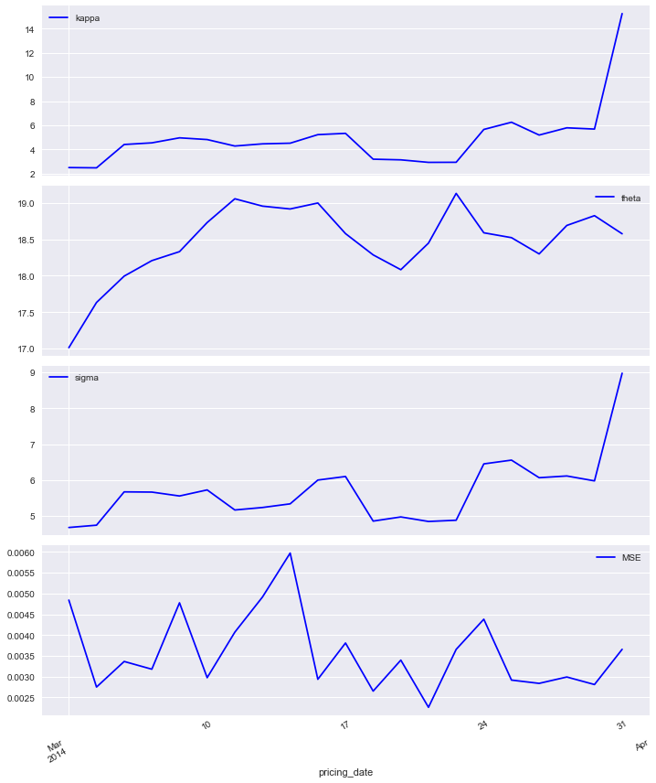
This is also illustrated by the visualization of the time series data for the calibrated/optimal parameter values. The MSE is below 0.01 throughout.
[22]:
%matplotlib inline
paramet[['kappa', 'theta', 'sigma', 'MSE']].plot(subplots=True, color='b', figsize=(10, 12))
plt.tight_layout()
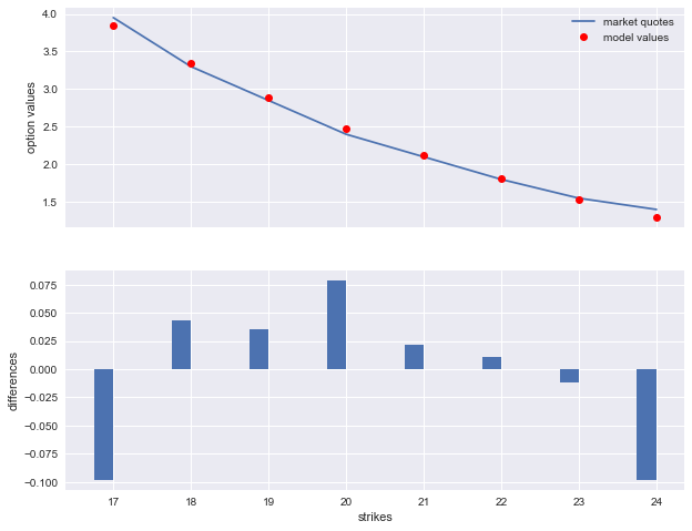
The following generates a plot of the calibration results for the last calibration day. The absolute price differences are below 0.10 EUR for all options.
[23]:
index = paramet.index[-1]
opt = np.array(paramet[['kappa', 'theta', 'sigma']].loc[index])
option_selection = get_option_selection(index, maturity_list[0], tol=tol)[0]
model_values = np.sort(np.array(list(calculate_model_values(opt).values())))[::-1]
import matplotlib.pyplot as plt
%matplotlib inline
fix, (ax1, ax2) = plt.subplots(2, sharex=True, figsize=(10, 8))
strikes = option_selection['STRIKE'].values
ax1.plot(strikes, option_selection['PRICE'], label='market quotes')
ax1.plot(strikes, model_values, 'ro', label='model values')
ax1.set_ylabel('option values')
ax1.grid(True)
ax1.legend(loc=0)
wi = 0.25
ax2.bar(strikes - wi / 2., model_values - option_selection['PRICE'],
        label='market quotes', width=wi)
ax2.grid(True)
ax2.set_ylabel('differences')
ax2.set_xlabel('strikes')
[23]:
<matplotlib.text.Text at 0x116ec0b00>
Copyright, License & Disclaimer
© Dr. Yves J. Hilpisch | The Python Quants GmbH
DX Analytics (the “dx library” or “dx package”) is licensed under the GNU Affero General Public License version 3 or later (see http://www.gnu.org/licenses/).
DX Analytics comes with no representations or warranties, to the extent permitted by applicable law.
http://tpq.io | dx@tpq.io | http://twitter.com/dyjh
Quant Platform | http://pqp.io
Python for Finance Training | http://training.tpq.io
Certificate in Computational Finance | http://compfinance.tpq.io
Derivatives Analytics with Python (Wiley Finance) | http://dawp.tpq.io
Python for Finance (2nd ed., O’Reilly) | http://py4fi.tpq.io