7. Parallel Valuation of Large Portfolios
Derivatives (portfolio) valuation by Monte Carlo simulation is a computationally demanding task. For practical applications, when valuation speed plays an important role, parallelization of both simulation and valuation tasks might prove a useful strategy. DX Analytics has built in a basic parallelization option which allows the use of the Python mulitprocessing module. Depending on the tasks at hand this can already lead to significant speed-ups.
[1]:
from dx import *
import time
from pylab import plt
plt.style.use('seaborn')
%matplotlib inline
7.1. Single Risk Factor
The example is based on a single risk factor, a geometric_brownian_motion object.
[2]:
# constant short rate
r = constant_short_rate('r', 0.02)
[3]:
# market environments
me_gbm = market_environment('gbm', dt.datetime(2015, 1, 1))
[4]:
# geometric Brownian motion
me_gbm.add_constant('initial_value', 100.)
me_gbm.add_constant('volatility', 0.2)
me_gbm.add_constant('currency', 'EUR')
me_gbm.add_constant('model', 'gbm')
[5]:
# valuation environment
val_env = market_environment('val_env', dt.datetime(2015, 1, 1))
val_env.add_constant('paths', 25000)
val_env.add_constant('frequency', 'M')
val_env.add_curve('discount_curve', r)
val_env.add_constant('starting_date', dt.datetime(2015, 1, 1))
val_env.add_constant('final_date', dt.datetime(2015, 12, 31))
[6]:
# add valuation environment to market environments
me_gbm.add_environment(val_env)
[7]:
risk_factors = {'gbm' : me_gbm}
7.2. American Put Option
We also model only a single derivative instrument.
[8]:
gbm = geometric_brownian_motion('gbm_obj', me_gbm)
[9]:
me_put = market_environment('put', dt.datetime(2015, 1, 1))
me_put.add_constant('maturity', dt.datetime(2015, 12, 31))
me_put.add_constant('strike', 40.)
me_put.add_constant('currency', 'EUR')
me_put.add_environment(val_env)
[10]:
am_put = valuation_mcs_american_single(
                'am_put', mar_env=me_put, underlying=gbm,
                payoff_func='np.maximum(strike - instrument_values, 0)')
7.3. Large Portfolio
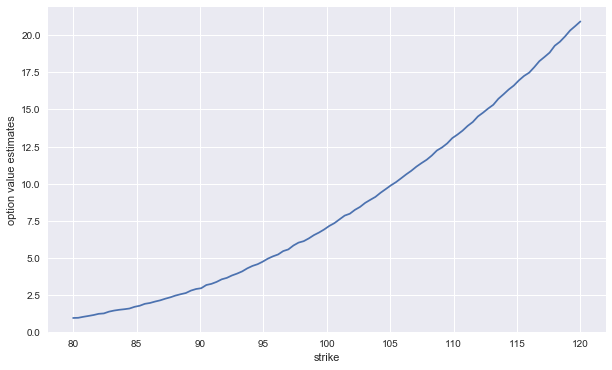
However, the derivatives_portfolio object we compose consists of 100 derivatives positions. Each option differes with respect to the strike.
[11]:
positions = {}
strikes = np.linspace(80, 120, 100)
for i, strike in enumerate(strikes):
    positions[i] = derivatives_position(
                        name='am_put_pos_%s' % strike,
                        quantity=1,
                        underlyings=['gbm'],
                        mar_env=me_put,
                        otype='American single',
        payoff_func='np.maximum(%5.3f - instrument_values, 0)' % strike)
7.3.1. Sequential Valuation
First, the derivatives portfolio with sequential valuation.
[12]:
port_sequ = derivatives_portfolio(
                name='portfolio',
                positions=positions,
                val_env=val_env,
                risk_factors=risk_factors,
                correlations=None,
                parallel=False)  # sequential calculation
The call of the get_values method to value all instruments …
[13]:
t0 = time.time()
ress = port_sequ.get_values()
ts = time.time() - t0
print('Time in sec %.2f' % ts)
Total
 pos_value    839.234
dtype: float64
Time in sec 4.09
… and the results visualized.
[14]:
ress['strike'] = strikes
ress.set_index('strike')['value'].plot(figsize=(10, 6))
plt.ylabel('option value estimates')
[14]:
Text(0,0.5,'option value estimates')
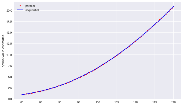
7.3.2. Parallel Valuation
Second, the derivatives portfolio with parallel valuation.
[15]:
port_para = derivatives_portfolio(
                'portfolio',
                positions,
                val_env,
                risk_factors,
                correlations=None,
                parallel=True)  # parallel valuation
The call of the get_values method for the parall valuation case.
[16]:
t0 = time.time()
resp = port_para.get_values()
  # parallel valuation with as many cores as available
tp = time.time() - t0
print('Time in sec %.2f' % tp)
Total
 pos_value    840.238
dtype: float64
Time in sec 5.36
Again, the results visualized (and compared to the sequential results).
[17]:
plt.figure(figsize=(10, 6))
plt.plot(strikes, resp['value'].values, 'r.', label='parallel')
plt.plot(strikes, ress['value'].values, 'b', label='sequential')
plt.legend(loc=0)
plt.ylabel('option value estimates')
[17]:
Text(0,0.5,'option value estimates')
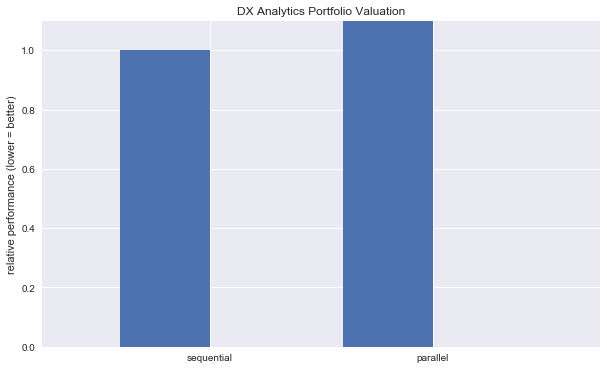
7.3.3. Speed-up
The realized speed-up is of course dependend on the hardware used, and in particular the number of cores (threads) available.
[18]:
ts / tp
  # speed-up factor
  # of course harware-dependent
[18]:
0.7630898756144515
[19]:
wi = 0.4
plt.figure(figsize=(10, 6))
plt.bar((1.5 - wi/2, 2.5 - wi/2), (ts/ts, tp/ts), width=wi)
plt.xticks((1.5, 2.5), ('sequential', 'parallel'))
plt.ylim(0, 1.1), plt.xlim(0.75, 3.25)
plt.ylabel('relative performance (lower = better)')
plt.title('DX Analytics Portfolio Valuation')
[19]:
Text(0.5,1,'DX Analytics Portfolio Valuation')
Copyright, License & Disclaimer
© Dr. Yves J. Hilpisch | The Python Quants GmbH
DX Analytics (the “dx library” or “dx package”) is licensed under the GNU Affero General Public License version 3 or later (see http://www.gnu.org/licenses/).
DX Analytics comes with no representations or warranties, to the extent permitted by applicable law.
http://tpq.io | dx@tpq.io | http://twitter.com/dyjh
Quant Platform | http://pqp.io
Python for Finance Training | http://training.tpq.io
Certificate in Computational Finance | http://compfinance.tpq.io
Derivatives Analytics with Python (Wiley Finance) | http://dawp.tpq.io
Python for Finance (2nd ed., O’Reilly) | http://py4fi.tpq.io