11. Interest Rate Swaps
Very nascent.
Interest rate swaps are a first step towards including rate-sensitive instruments in the modeling and valuation spectrum of DX Analytics. The model used in the following is the square-root diffusion process by Cox-Ingersoll-Ross (1985). Data used are UK/London OIS and Libor rates.
[1]:
import dx
import time
import numpy as np
import pandas as pd
import datetime as dt
from pylab import plt
plt.style.use('seaborn')
%matplotlib inline
11.1. OIS Data & Discounting
We start by importing OIS term structure data (source: http://www.bankofengland.co.uk) for risk-free discounting. We also adjust the data structure somewhat for our purposes.
[2]:
# UK OIS Spot Rates Yield Curve
oiss = pd.read_excel('data/ukois09.xls', 'oiss')
# use years as index
oiss = oiss.set_index('years')
# del oiss['years']
[3]:
# only date information for columns, no time
oiss.columns = [d.date() for d in oiss.columns]
[4]:
oiss.tail()
[4]:
| 2014-10-01 | 2014-10-02 | 2014-10-03 | 2014-10-06 | 2014-10-07 | 2014-10-08 | 2014-10-09 | 2014-10-10 | 2014-10-13 | 2014-10-14 | 2014-10-15 | 2014-10-16 | |
|---|---|---|---|---|---|---|---|---|---|---|---|---|
| years | ||||||||||||
| 4.666667 | 1.550947 | 1.525838 | 1.570203 | 1.533901 | 1.479044 | 1.445234 | 1.436023 | 1.409962 | 1.337567 | 1.283932 | 1.063205 | 1.234125 |
| 4.750000 | 1.563661 | 1.538616 | 1.583198 | 1.546459 | 1.491152 | 1.457593 | 1.448627 | 1.422015 | 1.349782 | 1.296052 | 1.074773 | 1.246277 |
| 4.833333 | 1.576142 | 1.551158 | 1.595952 | 1.558789 | 1.503050 | 1.469768 | 1.461040 | 1.433887 | 1.361832 | 1.308025 | 1.086254 | 1.258307 |
| 4.916667 | 1.588400 | 1.563474 | 1.608472 | 1.570898 | 1.514746 | 1.481764 | 1.473269 | 1.445585 | 1.373724 | 1.319859 | 1.097650 | 1.270219 |
| 5.000000 | 1.600442 | 1.575572 | 1.620768 | 1.582794 | 1.526247 | 1.493588 | 1.485320 | 1.457116 | 1.385461 | 1.331557 | 1.108962 | 1.282014 |
Next we replace the year fraction index by a DatetimeIndex.
[5]:
# generate time index given input data
# starting date + 59 months
date = oiss.columns[-1]
index = pd.date_range(date, periods=60, freq='M') # , tz='GMT')
index = [d.replace(day=date.day) for d in index]
index = pd.DatetimeIndex(index)
oiss.index = index
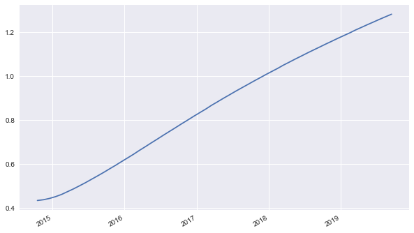
Let us have a look at the most current data, i.e. the term structure, of the data set.
[6]:
oiss.iloc[:, -1].plot(figsize=(10, 6))
[6]:
<matplotlib.axes._subplots.AxesSubplot at 0x10ba062b0>
This data is used to instantiate a deterministic_short_rate model for risk-neutral discounting purposes.
[7]:
# generate deterministic short rate model based on UK OIS curve
ois = dx.deterministic_short_rate('ois', list(zip(oiss.index, oiss.iloc[:, -1].values / 100)))
[8]:
# example dates and corresponding discount factors
dr = pd.date_range('2015-1', periods=4, freq='6m').to_pydatetime()
ois.get_discount_factors(dr)[::-1]
[8]:
([0.989825148692371, 0.9922754901627036, 0.9956237774158325, 1.0],
 array([datetime.datetime(2015, 1, 31, 0, 0),
        datetime.datetime(2015, 7, 31, 0, 0),
        datetime.datetime(2016, 1, 31, 0, 0),
        datetime.datetime(2016, 7, 31, 0, 0)], dtype=object))
11.2. Libor Market Data
We want to model a 3 month Libor-based interest rate swap. To this end, we need Libor term structure data, i.e. forward rates in this case (source: http://www.bankofengland.co.uk), to calibrate the valuation to. The data importing and adjustments are the same as before.
[9]:
# UK Libor foward rates
libf = pd.read_excel('data/ukblc05.xls', 'fwds')
# use years as index
libf = libf.set_index('years')
[10]:
# only date information for columns, no time
libf.columns = [d.date() for d in libf.columns]
[11]:
libf.tail()
[11]:
| 2014-10-01 | 2014-10-02 | 2014-10-03 | 2014-10-06 | 2014-10-07 | 2014-10-08 | 2014-10-09 | 2014-10-10 | 2014-10-13 | 2014-10-14 | 2014-10-15 | 2014-10-16 | |
|---|---|---|---|---|---|---|---|---|---|---|---|---|
| years | ||||||||||||
| 4.666667 | 2.722915 | 2.686731 | 2.678433 | 2.681385 | 2.639166 | 2.542012 | 2.528768 | 2.489063 | 2.470154 | 2.349732 | 2.372435 | 2.157431 |
| 4.750000 | 2.733588 | 2.697887 | 2.690366 | 2.692824 | 2.650841 | 2.554583 | 2.543066 | 2.502357 | 2.483842 | 2.366052 | 2.387671 | 2.176186 |
| 4.833333 | 2.744126 | 2.708848 | 2.702083 | 2.704147 | 2.662380 | 2.567071 | 2.557216 | 2.515531 | 2.497446 | 2.382298 | 2.402829 | 2.194784 |
| 4.916667 | 2.754540 | 2.719634 | 2.713604 | 2.715368 | 2.673794 | 2.579486 | 2.571229 | 2.528592 | 2.510973 | 2.398468 | 2.417915 | 2.213221 |
| 5.000000 | 2.764842 | 2.730264 | 2.724949 | 2.726501 | 2.685095 | 2.591835 | 2.585117 | 2.541548 | 2.524432 | 2.414562 | 2.432939 | 2.231493 |
[12]:
# generate time index given input data
# starting date + 59 months
date = libf.columns[-1]
index = pd.date_range(date, periods=60, freq='M')  # , tz='GMT')
index = [d.replace(day=date.day) for d in index]
index = pd.DatetimeIndex(index)
libf.index = index
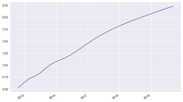
And the short end of the Libor term sturcture visualized.
[13]:
libf.iloc[:, -1].plot(figsize=(10, 6))
[13]:
<matplotlib.axes._subplots.AxesSubplot at 0x10bfe8198>
11.3. Model Calibration
Next, equipped with the Libor data, we calibrate the square-root diffusion short rate model. A bit of data preparation:
[14]:
t = libf.index.to_pydatetime()
f = libf.iloc[:, -1].values / 100
initial_value = 0.005
A mean-squared error (MSE) function to be minimized during calibration.
[15]:
def srd_forward_error(p0):
    global initial_value, f, t
    if p0[0] < 0 or p0[1] < 0 or p0[2] < 0:
        return 100
    f_model = dx.srd_forwards(initial_value, p0, t)
    MSE = np.sum((f - f_model) ** 2) / len(f)
    return MSE
And the calibration itself.
[16]:
from scipy.optimize import fmin
[17]:
opt = fmin(srd_forward_error, (1.0, 0.7, 0.2),
           maxiter=1000, maxfun=1000)
Optimization terminated successfully.
         Current function value: 0.000000
         Iterations: 371
         Function evaluations: 649
The optimal parameters (kappa, theta, sigma) are:
[18]:
opt
[18]:
array([0.00544441, 1.80697228, 0.23689443])
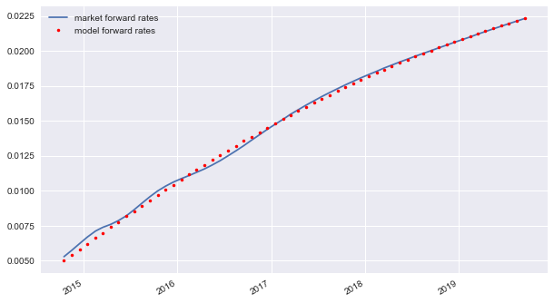
The model fit is not too bad in this case.
[19]:
plt.figure(figsize=(10, 6))
plt.plot(t, f, label='market forward rates')
plt.plot(t, dx.srd_forwards(initial_value, opt, t), 'r.', label='model forward rates')
plt.gcf().autofmt_xdate(); plt.legend(loc=0)
[19]:
<matplotlib.legend.Legend at 0x10bfbcef0>
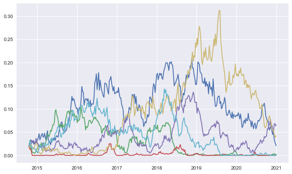
11.4. Floating Rate Modeling
The optimal parameters from the calibration are used to model the floating rate (3m Libor rate).
[20]:
# market environment
me_srd = dx.market_environment('me_srd', dt.datetime(2014, 10, 16))
[21]:
# square-root diffusion
me_srd.add_constant('initial_value', 0.02)
me_srd.add_constant('kappa', opt[0])
me_srd.add_constant('theta', opt[1])
me_srd.add_constant('volatility', opt[2])
me_srd.add_curve('discount_curve', ois)
  # OIS discounting object
me_srd.add_constant('currency', 'EUR')
me_srd.add_constant('paths', 10000)
me_srd.add_constant('frequency', 'w')
me_srd.add_constant('starting_date', me_srd.pricing_date)
me_srd.add_constant('final_date', dt.datetime(2020, 12, 31))
[22]:
srd = dx.square_root_diffusion('srd', me_srd)
Let us have a look at some simulated rate paths.
[23]:
paths = srd.get_instrument_values()
[24]:
plt.figure(figsize=(10, 6))
plt.plot(srd.time_grid, paths[:, :6])
[24]:
[<matplotlib.lines.Line2D at 0x10ba7de10>,
 <matplotlib.lines.Line2D at 0x10c2f6400>,
 <matplotlib.lines.Line2D at 0x10c2f6668>,
 <matplotlib.lines.Line2D at 0x10c2f6898>,
 <matplotlib.lines.Line2D at 0x10c2f6ac8>,
 <matplotlib.lines.Line2D at 0x10c2f6cf8>]
11.5. Interest Rate Swap
Finally, we can model the interest rate swap itself.
11.5.1. Modeling
First, the market environment with all the parameters needed.
[25]:
# market environment for the IRS
me_irs = dx.market_environment('irs', me_srd.pricing_date)
me_irs.add_constant('fixed_rate', 0.01)
me_irs.add_constant('trade_date', me_srd.pricing_date)
me_irs.add_constant('effective_date', me_srd.pricing_date)
me_irs.add_constant('payment_date', dt.datetime(2014, 12, 27))
me_irs.add_constant('payment_day', 27)
me_irs.add_constant('termination_date', me_srd.get_constant('final_date'))
me_irs.add_constant('currency', 'EUR')
me_irs.add_constant('notional', 1000000)
me_irs.add_constant('tenor', '6m')
me_irs.add_constant('counting', 'ACT/360')
# discount curve from mar_env of floating rate
The instantiation of the valuation object.
[26]:
irs = dx.interest_rate_swap('irs', srd, me_irs)
11.5.2. Valuation
The present value of the interest rate swap given the assumption, in particular, of the fixed rate.
[27]:
%time irs.present_value(fixed_seed=True)
CPU times: user 198 ms, sys: 82 ms, total: 280 ms
Wall time: 299 ms
[27]:
482804.6280483039
You can also generate a full output of all present values per simulation path.
[28]:
irs.present_value(full=True).iloc[:, :6]
[28]:
| 0 | 1 | 2 | 3 | 4 | 5 | |
|---|---|---|---|---|---|---|
| 2014-12-27 | 20919.908406 | 3765.545880 | -10000.000000 | 20447.662984 | 15671.171542 | -461.905549 |
| 2015-06-27 | 27796.391566 | 67649.371268 | -7952.865109 | 21069.238749 | 6547.642190 | 56254.997722 |
| 2015-12-27 | 72797.267752 | 65085.851729 | -9495.534310 | 7184.517383 | -6249.109421 | 72603.409748 |
| 2016-06-27 | 146587.773739 | 60725.900678 | -9450.695252 | 10630.874710 | 1457.279233 | 96390.826927 |
| 2016-12-27 | 112006.856512 | 11685.574401 | -9365.011855 | 36777.060898 | 40752.233786 | 42437.807055 |
| 2017-06-27 | 89091.008350 | 19143.973791 | -8652.442452 | 10394.933700 | 81112.588234 | 49316.809090 |
| 2017-12-27 | 153802.099096 | 37433.554707 | -2231.031239 | 3046.024441 | 81218.496071 | 89235.982850 |
| 2018-06-27 | 114033.046751 | -4200.273599 | 8204.181410 | 86020.232903 | 92146.494366 | 44010.774119 |
| 2018-12-27 | 165327.788708 | -7186.102024 | -8829.883386 | 46785.300398 | 171037.865434 | 14615.688086 |
| 2019-06-27 | 101110.008932 | -9038.246291 | -6883.724709 | 29794.380064 | 183168.704902 | -4599.638746 |
| 2019-12-27 | 57890.028467 | -8998.424023 | -8573.907447 | 12491.846129 | 151080.678798 | -8960.333669 |
| 2020-06-27 | 95516.235053 | -8968.295497 | -8963.127240 | 15234.994497 | 67282.503413 | -7763.697572 |
| 2020-12-27 | 4651.947620 | -4500.468014 | -6316.280222 | 39899.010233 | 107971.761933 | -8568.679338 |
Copyright, License & Disclaimer
© Dr. Yves J. Hilpisch | The Python Quants GmbH
DX Analytics (the “dx library” or “dx package”) is licensed under the GNU Affero General Public License version 3 or later (see http://www.gnu.org/licenses/).
DX Analytics comes with no representations or warranties, to the extent permitted by applicable law.
http://tpq.io | dx@tpq.io | http://twitter.com/dyjh
Quant Platform | http://pqp.io
Python for Finance Training | http://training.tpq.io
Certificate in Computational Finance | http://compfinance.tpq.io
Derivatives Analytics with Python (Wiley Finance) | http://dawp.tpq.io
Python for Finance (2nd ed., O’Reilly) | http://py4fi.tpq.io