12. Mean-Variance Portfolio Class
Without doubt, the Markowitz (1952) mean-variance portfolio theory is a cornerstone of modern financial theory. This section illustrates the use of the mean_variance_portfolio class to implement this approach.
[1]:
from dx import *
from pylab import plt
plt.style.use('seaborn')
12.1. Market Environment and Portfolio Object
We start by instantiating a market environment object which in particular contains a list of ticker symbols in which we are interested in.
[11]:
ma = market_environment('ma', dt.date(2010, 1, 1))
ma.add_list('symbols', ['AAPL.O', 'INTC.O', 'MSFT.O', 'GS.N'])
ma.add_constant('source', 'google')
ma.add_constant('final date', dt.date(2014, 3, 1))
Using pandas under the hood, the class retrieves historial stock price data from either Yahoo! Finance of Google.
[13]:
%%time
port = mean_variance_portfolio('am_tech_stocks', ma)
  # instantiates the portfolio class
  # and retrieves all the time series data needed
CPU times: user 16.1 ms, sys: 4.44 ms, total: 20.5 ms
Wall time: 179 ms
[14]:
port.get_available_symbols()
[14]:
Index(['AAPL.O', 'MSFT.O', 'INTC.O', 'AMZN.O', 'GS.N', 'SPY', '.SPX', '.VIX',
       'EUR=', 'XAU=', 'GDX', 'GLD'],
      dtype='object')
12.2. Basic Statistics
Since no portfolio weights have been provided, the class defaults to equal weights.
[15]:
port.get_weights()
  # defaults to equal weights
[15]:
{'AAPL.O': 0.25, 'GS.N': 0.25, 'INTC.O': 0.25, 'MSFT.O': 0.25}
Given these weights you can calculate the portfolio return via the method get_portfolio_return.
[16]:
port.get_portfolio_return()
  # expected (= historical mean) return
[16]:
0.12192541796457722
Analogously, you can call get_portfolio_variance to get the historical portfolio variance.
[17]:
port.get_portfolio_variance()
  # expected (= historical) variance
[17]:
0.03365126396235786
The class also has a neatly printable string representation.
[18]:
print(port)
  # ret. con. is "return contribution"
  # given the mean return and the weight
  # of the security
Portfolio am_tech_stocks
--------------------------
return            0.122
volatility        0.183
Sharpe ratio      0.665

Positions
symbol | weight | ret. con.
---------------------------
AAPL.O |  0.250 |     0.055
INTC.O |  0.250 |     0.025
MSFT.O |  0.250 |     0.032
GS.N   |  0.250 |     0.011
12.3. Setting Weights
Via the method set_weights the weights of the single portfolio components can be adjusted.
[19]:
port.set_weights([0.6, 0.2, 0.1, 0.1])
[21]:
print(port)
Portfolio am_tech_stocks
--------------------------
return            0.168
volatility        0.201
Sharpe ratio      0.837

Positions
symbol | weight | ret. con.
---------------------------
AAPL.O |  0.600 |     0.131
INTC.O |  0.200 |     0.020
MSFT.O |  0.100 |     0.013
GS.N   |  0.100 |     0.004
You cal also easily check results for different weights with changing the attribute values of an object.
[22]:
port.test_weights([0.6, 0.2, 0.1, 0.1])
    # returns av. return + vol + Sharp ratio
    # without setting new weights
[22]:
array([0.16804275, 0.20076851, 0.83699753])
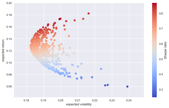
Let us implement a Monte Carlo simulation over potential portfolio weights.
[23]:
# Monte Carlo simulation of portfolio compositions
rets = []
vols = []

for w in range(500):
    weights = np.random.random(4)
    weights /= sum(weights)
    r, v, sr = port.test_weights(weights)
    rets.append(r)
    vols.append(v)

rets = np.array(rets)
vols = np.array(vols)
And the simulation results visualized.
[29]:
import matplotlib.pyplot as plt
%matplotlib inline
plt.figure(figsize=(10, 6))
plt.scatter(vols, rets, c=rets / vols, marker='o', cmap='coolwarm')
plt.xlabel('expected volatility')
plt.ylabel('expected return')
plt.colorbar(label='Sharpe ratio');
12.4. Optimizing Portfolio Composition
One of the major application areas of the mean-variance portfolio theory and therewith of this DX Analytics class it the optimization of the portfolio composition. Different target functions can be used to this end.
12.4.1. Return
The first target function might be the portfolio return.
[30]:
port.optimize('Return')
  # maximizes expected return of portfolio
  # no volatility constraint
[31]:
print(port)
Portfolio am_tech_stocks
--------------------------
return            0.219
volatility        0.255
Sharpe ratio      0.858

Positions
symbol | weight | ret. con.
---------------------------
AAPL.O |  1.000 |     0.219
INTC.O |  0.000 |     0.000
MSFT.O |  0.000 |     0.000
GS.N   |  0.000 |     0.000
Instead of maximizing the portfolio return without any constraints, you can also set a (sensible/possible) maximum target volatility level as a constraint. Both, in an exact sense (“equality constraint”) …
[32]:
port.optimize('Return', constraint=0.225, constraint_type='Exact')
  # interpretes volatility constraint as equality
[33]:
print(port)
Portfolio am_tech_stocks
--------------------------
return            0.095
volatility        0.225
Sharpe ratio      0.421

Positions
symbol | weight | ret. con.
---------------------------
AAPL.O |  0.294 |     0.064
INTC.O |  0.000 |     0.000
MSFT.O |  0.000 |     0.000
GS.N   |  0.706 |     0.030
… or just a an upper bound (“inequality constraint”).
[34]:
port.optimize('Return', constraint=0.4, constraint_type='Bound')
  # interpretes volatility constraint as inequality (upper bound)
[35]:
print(port)
Portfolio am_tech_stocks
--------------------------
return            0.219
volatility        0.255
Sharpe ratio      0.858

Positions
symbol | weight | ret. con.
---------------------------
AAPL.O |  1.000 |     0.219
INTC.O |  0.000 |     0.000
MSFT.O |  0.000 |     0.000
GS.N   |  0.000 |     0.000
12.4.2. Risk
The class also allows you to minimize portfolio risk.
[36]:
port.optimize('Vol')
  # minimizes expected volatility of portfolio
  # no return constraint
[37]:
print(port)
Portfolio am_tech_stocks
--------------------------
return            0.128
volatility        0.182
Sharpe ratio      0.702

Positions
symbol | weight | ret. con.
---------------------------
AAPL.O |  0.250 |     0.055
INTC.O |  0.275 |     0.027
MSFT.O |  0.305 |     0.039
GS.N   |  0.169 |     0.007
And, as before, to set constraints (in this case) for the target return level.
[38]:
port.optimize('Vol', constraint=0.175, constraint_type='Exact')
  # interpretes return constraint as equality
[39]:
print(port)
Portfolio am_tech_stocks
--------------------------
return            0.175
volatility        0.199
Sharpe ratio      0.879

Positions
symbol | weight | ret. con.
---------------------------
AAPL.O |  0.561 |     0.123
INTC.O |  0.118 |     0.012
MSFT.O |  0.321 |     0.041
GS.N   |  0.000 |     0.000
[40]:
port.optimize('Vol', constraint=0.20, constraint_type='Bound')
  # interpretes return constraint as inequality (upper bound)
[41]:
print(port)
Portfolio am_tech_stocks
--------------------------
return            0.200
volatility        0.225
Sharpe ratio      0.889

Positions
symbol | weight | ret. con.
---------------------------
AAPL.O |  0.798 |     0.174
INTC.O |  0.000 |     0.000
MSFT.O |  0.202 |     0.026
GS.N   |  0.000 |     0.000
12.4.3. Sharpe Ratio
Often, the target of the portfolio optimization efforts is the so called Sharpe ratio. The mean_variance_portfolio class of DX Analytics assumes a risk-free rate of zero in this context.
[42]:
port.optimize('Sharpe')
  # maximize Sharpe ratio
[43]:
print(port)
Portfolio am_tech_stocks
--------------------------
return            0.192
volatility        0.215
Sharpe ratio      0.893

Positions
symbol | weight | ret. con.
---------------------------
AAPL.O |  0.713 |     0.156
INTC.O |  0.000 |     0.000
MSFT.O |  0.287 |     0.036
GS.N   |  0.000 |     0.000
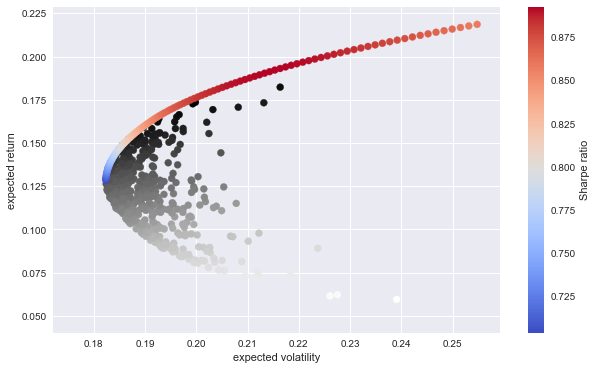
12.5. Efficient Frontier
Another application area is to derive the efficient frontier in the mean-variance space. These are all these portfolios for which there is no portfolio with both lower risk and higher return. The method get_efficient_frontier yields the desired results.
[44]:
%%time
evols, erets = port.get_efficient_frontier(100)
  # 100 points of the effient frontier
CPU times: user 4.24 s, sys: 10.8 ms, total: 4.25 s
Wall time: 4.25 s
The plot with the random and efficient portfolios.
[46]:
plt.figure(figsize=(10, 6))
plt.scatter(vols, rets, c=rets / vols, marker='o')
plt.scatter(evols, erets, c=erets / evols, marker='o', cmap='coolwarm')
plt.xlabel('expected volatility')
plt.ylabel('expected return')
plt.colorbar(label='Sharpe ratio')
[46]:
<matplotlib.colorbar.Colorbar at 0x10f8dc550>
12.6. Capital Market Line
The capital market line is another key element of the mean-variance portfolio approach representing all those risk-return combinations (in mean-variance space) that are possible to form from a risk-less money market account and the market portfolio (or another appropriate substitute efficient portfolio).
[47]:
%%time
cml, optv, optr = port.get_capital_market_line(riskless_asset=0.05)
  # capital market line for effiecient frontier and risk-less short rate
CPU times: user 4.04 s, sys: 4.81 ms, total: 4.05 s
Wall time: 4.05 s
[48]:
cml # lambda function for capital market line
[48]:
<function dx.portfolio.mean_variance_portfolio.get_capital_market_line.<locals>.<lambda>>
The following plot illustrates that the capital market line has an ordinate value equal to the risk-free rate (the safe return of the money market account) and is tangent to the efficient frontier.
[49]:
plt.figure(figsize=(10, 6))
plt.plot(evols, erets, lw=2.0, label='efficient frontier')
plt.plot((0, 0.4), (cml(0), cml(0.4)), lw=2.0, label='capital market line')
plt.plot(optv, optr, 'r*', markersize=10, label='optimal portfolio')
plt.legend(loc=0)
plt.ylim(0)
plt.xlabel('expected volatility')
plt.ylabel('expected return')
[49]:
<matplotlib.text.Text at 0x10f3809e8>
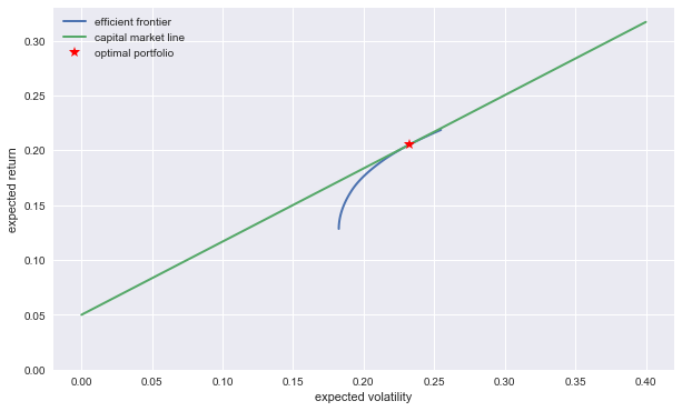
Portfolio return and risk of the efficient portfolio used are:
[50]:
optr
[50]:
0.20507680142118542
[51]:
optv
[51]:
0.23227456779433622
The portfolio composition can be derived as follows.
[52]:
port.optimize('Vol', constraint=optr, constraint_type='Exact')
[53]:
print(port)
Portfolio am_tech_stocks
--------------------------
return            0.205
volatility        0.232
Sharpe ratio      0.883

Positions
symbol | weight | ret. con.
---------------------------
AAPL.O |  0.853 |     0.186
INTC.O |  0.000 |     0.000
MSFT.O |  0.147 |     0.019
GS.N   |  0.000 |     0.000
Or also in this way.
[54]:
port.optimize('Return', constraint=optv, constraint_type='Exact')
[55]:
print(port)
Portfolio am_tech_stocks
--------------------------
return            0.083
volatility        0.232
Sharpe ratio      0.357

Positions
symbol | weight | ret. con.
---------------------------
AAPL.O |  0.226 |     0.050
INTC.O |  0.000 |     0.000
MSFT.O |  0.000 |     0.000
GS.N   |  0.774 |     0.033
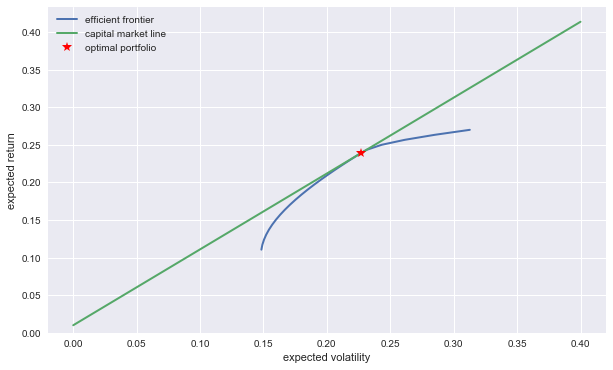
12.7. More Assets
As a larger, more realistic example, consider a larger set of assets.
[71]:
symbols = list(port.get_available_symbols())[:7]
symbols
[71]:
['AAPL.O', 'MSFT.O', 'INTC.O', 'AMZN.O', 'GS.N', 'SPY', '.SPX']
[72]:
ma = market_environment('ma', dt.date(2010, 1, 1))
ma.add_list('symbols', symbols)
ma.add_constant('source', 'google')
ma.add_constant('final date', dt.date(2014, 3, 1))
Data retrieval in this case takes a bit.
[73]:
%%time
djia = mean_variance_portfolio('djia', ma)
  # defining the portfolio and retrieving the data
CPU times: user 14.2 ms, sys: 4.63 ms, total: 18.8 ms
Wall time: 212 ms
[74]:
%%time
djia.optimize('Vol')
print(djia.variance, djia.variance ** 0.5)
  # minimium variance & volatility in decimals
0.021982829770393886 0.14826607761181884
CPU times: user 55.8 ms, sys: 1.83 ms, total: 57.6 ms
Wall time: 56.1 ms
Given the larger data set now used, efficient frontier …
[75]:
%%time
evols, erets = djia.get_efficient_frontier(25)
  # efficient frontier of DJIA
CPU times: user 2.28 s, sys: 3.93 ms, total: 2.28 s
Wall time: 2.28 s
… and capital market line derivations take also longer.
[76]:
%%time
cml, optv, optr = djia.get_capital_market_line(riskless_asset=0.01)
  # capital market line and optimal (tangent) portfolio
CPU times: user 8.4 s, sys: 6.07 ms, total: 8.4 s
Wall time: 8.4 s
[77]:
plt.figure(figsize=(10, 6))
plt.plot(evols, erets, lw=2.0, label='efficient frontier')
plt.plot((0, 0.4), (cml(0), cml(0.4)), lw=2.0, label='capital market line')
plt.plot(optv, optr, 'r*', markersize=10, label='optimal portfolio')
plt.legend(loc=0)
plt.ylim(0)
plt.xlabel('expected volatility')
plt.ylabel('expected return')
[77]:
<matplotlib.text.Text at 0x1103a70b8>
Copyright, License & Disclaimer
© Dr. Yves J. Hilpisch | The Python Quants GmbH
DX Analytics (the “dx library” or “dx package”) is licensed under the GNU Affero General Public License version 3 or later (see http://www.gnu.org/licenses/).
DX Analytics comes with no representations or warranties, to the extent permitted by applicable law.
http://tpq.io | dx@tpq.io | http://twitter.com/dyjh
Quant Platform | http://pqp.io
Python for Finance Training | http://training.tpq.io
Certificate in Computational Finance | http://compfinance.tpq.io
Derivatives Analytics with Python (Wiley Finance) | http://dawp.tpq.io
Python for Finance (2nd ed., O’Reilly) | http://py4fi.tpq.io