14. Quite Complex Portfolios
This part illustrates that you can model, value and risk manage quite complex derivatives portfolios with DX Analytics.
[1]:
from dx import *
import time
from pylab import plt
plt.style.use('seaborn')
%matplotlib inline
np.random.seed(10000)
14.1. Multiple Risk Factors
The example is based on a multiple, correlated risk factors, all (for the ease of exposition) geometric_brownian_motion objects.
[2]:
mer = market_environment(name='me', pricing_date=dt.datetime(2015, 1, 1))
mer.add_constant('initial_value', 0.01)
mer.add_constant('volatility', 0.1)
mer.add_constant('kappa', 2.0)
mer.add_constant('theta', 0.05)
mer.add_constant('paths', 100) # dummy
mer.add_constant('frequency', 'M') # dummy
mer.add_constant('starting_date', mer.pricing_date)
mer.add_constant('final_date', dt.datetime(2015, 12, 31)) # dummy
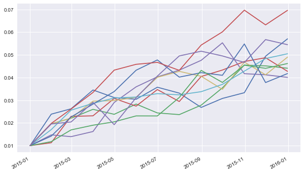
ssr = stochastic_short_rate('ssr', mer)
[3]:
plt.figure(figsize=(10, 6))
plt.plot(ssr.process.time_grid, ssr.process.get_instrument_values()[:, :10]);
plt.gcf().autofmt_xdate()
[4]:
# market environments
me = market_environment('gbm', dt.datetime(2015, 1, 1))
[5]:
# geometric Brownian motion
me.add_constant('initial_value', 36.)
me.add_constant('volatility', 0.2)
me.add_constant('currency', 'EUR')
[6]:
# jump diffusion
me.add_constant('lambda', 0.4)
me.add_constant('mu', -0.4)
me.add_constant('delta', 0.2)
[7]:
# stochastic volatility
me.add_constant('kappa', 2.0)
me.add_constant('theta', 0.3)
me.add_constant('vol_vol', 0.5)
me.add_constant('rho', -0.5)
Using 2,500 paths and monthly discretization for the example.
[8]:
# valuation environment
val_env = market_environment('val_env', dt.datetime(2015, 1, 1))
val_env.add_constant('paths', 1000)
val_env.add_constant('frequency', 'M')
val_env.add_curve('discount_curve', ssr)
val_env.add_constant('starting_date', dt.datetime(2015, 1, 1))
val_env.add_constant('final_date', dt.datetime(2016, 12, 31))
[9]:
# add valuation environment to market environments
me.add_environment(val_env)
[10]:
no = 50 # 50 different risk factors in total
[11]:
risk_factors = {}
for rf in range(no):
    # random model choice
    sm = np.random.choice(['gbm', 'jd', 'sv'])
    key = '%3d_%s' % (rf + 1, sm)
    risk_factors[key] = market_environment(key, me.pricing_date)
    risk_factors[key].add_environment(me)
    # random initial_value
    risk_factors[key].add_constant('initial_value',
                                    np.random.random() * 40. + 20.)
    # radnom volatility
    risk_factors[key].add_constant('volatility',
                                    np.random.random() * 0.6 + 0.05)
    # the simulation model to choose
    risk_factors[key].add_constant('model', sm)
[12]:
correlations = []
keys = sorted(risk_factors.keys())
for key in keys[1:]:
    correlations.append([keys[0], key, np.random.choice([-0.1, 0.0, 0.1])])
correlations[:3]
[12]:
[['  1_sv', '  2_gbm', 0.1],
 ['  1_sv', '  3_gbm', -0.1],
 ['  1_sv', '  4_gbm', -0.1]]
14.2. Options Modeling
We model a certain number of derivative instruments with the following major assumptions.
[13]:
me_option = market_environment('option', me.pricing_date)
# choose from a set of maturity dates (month ends)
maturities = pd.date_range(start=me.pricing_date,
                           end=val_env.get_constant('final_date'),
                           freq='M').to_pydatetime()
me_option.add_constant('maturity', np.random.choice(maturities))
me_option.add_constant('currency', 'EUR')
me_option.add_environment(val_env)
14.3. Portfolio Modeling
The derivatives_portfolio object we compose consists of multiple derivatives positions. Each option differs with respect to the strike and the risk factor it is dependent on.
[14]:
# 5 times the number of risk factors
# as portfolio positions/instruments
pos = 5 * no
[15]:
positions = {}
for i in range(pos):
    ot = np.random.choice(['am_put', 'eur_call'])
    if ot == 'am_put':
        otype = 'American single'
        payoff_func = 'np.maximum(%5.3f - instrument_values, 0)'
    else:
        otype = 'European single'
        payoff_func = 'np.maximum(maturity_value - %5.3f, 0)'
    # random strike
    strike = np.random.randint(36, 40)
    underlying = sorted(risk_factors.keys())[(i + no) % no]
    name = '%d_option_pos_%d' % (i, strike)
    positions[name] = derivatives_position(
                        name=name,
                        quantity=np.random.randint(1, 10),
                        underlyings=[underlying],
                        mar_env=me_option,
                        otype=otype,
        payoff_func=payoff_func % strike)
[16]:
# number of derivatives positions
len(positions)
[16]:
250
14.4. Portfolio Valuation
First, the derivatives portfolio with sequential valuation.
[17]:
port = derivatives_portfolio(
                name='portfolio',
                positions=positions,
                val_env=val_env,
                risk_factors=risk_factors,
                correlations=correlations,
                parallel=False)  # sequential calculation
[18]:
port.val_env.get_list('cholesky_matrix')
[18]:
array([[ 1.        ,  0.        ,  0.        , ...,  0.        ,
         0.        ,  0.        ],
       [ 0.1       ,  0.99498744,  0.        , ...,  0.        ,
         0.        ,  0.        ],
       [-0.1       ,  0.01005038,  0.99493668, ...,  0.        ,
         0.        ,  0.        ],
       ...,
       [-0.1       ,  0.01005038, -0.01015242, ...,  0.99239533,
         0.        ,  0.        ],
       [ 0.        ,  0.        ,  0.        , ...,  0.        ,
         1.        ,  0.        ],
       [ 0.1       , -0.01005038,  0.01015242, ...,  0.01526762,
         0.        ,  0.99227788]])
The call of the get_values method to value all instruments.
[19]:
%time res = port.get_statistics(fixed_seed=True)
Totals
 pos_value    10400.2920
pos_delta      116.0584
pos_vega      8477.9800
dtype: float64
CPU times: user 19.8 s, sys: 1.82 s, total: 21.6 s
Wall time: 15.4 s
[20]:
res.set_index('position', inplace=False)
[20]:
| name | quantity | otype | risk_facts | value | currency | pos_value | pos_delta | pos_vega | |
|---|---|---|---|---|---|---|---|---|---|
| position | |||||||||
| 0_option_pos_38 | 0_option_pos_38 | 6 | European single | [ 1_sv] | 7.263 | EUR | 43.578 | 3.6036 | 22.7046 |
| 1_option_pos_39 | 1_option_pos_39 | 8 | American single | [ 2_gbm] | 5.398 | EUR | 43.184 | -3.9168 | 124.5688 |
| 2_option_pos_37 | 2_option_pos_37 | 3 | European single | [ 3_gbm] | 3.306 | EUR | 9.918 | 1.9935 | 42.8949 |
| 3_option_pos_37 | 3_option_pos_37 | 8 | American single | [ 4_gbm] | 9.097 | EUR | 72.776 | -8.0000 | 5.3336 |
| 4_option_pos_39 | 4_option_pos_39 | 1 | European single | [ 5_gbm] | 17.664 | EUR | 17.664 | 0.7531 | 13.4445 |
| 5_option_pos_37 | 5_option_pos_37 | 3 | American single | [ 6_jd] | 13.354 | EUR | 40.062 | -3.0000 | 21.9111 |
| 6_option_pos_36 | 6_option_pos_36 | 9 | European single | [ 7_jd] | 17.651 | EUR | 158.859 | 7.9128 | 41.3010 |
| 7_option_pos_39 | 7_option_pos_39 | 3 | American single | [ 8_gbm] | 9.538 | EUR | 28.614 | -2.9169 | -4.6260 |
| 8_option_pos_36 | 8_option_pos_36 | 4 | American single | [ 9_sv] | 2.584 | EUR | 10.336 | -0.5512 | 5.1040 |
| 9_option_pos_39 | 9_option_pos_39 | 7 | American single | [ 10_sv] | 9.945 | EUR | 69.615 | -3.2571 | -1.2845 |
| 10_option_pos_37 | 10_option_pos_37 | 9 | European single | [ 11_jd] | 13.708 | EUR | 123.372 | 7.4493 | 70.9308 |
| 11_option_pos_38 | 11_option_pos_38 | 1 | European single | [ 12_jd] | 1.247 | EUR | 1.247 | 0.2810 | 8.4409 |
| 12_option_pos_38 | 12_option_pos_38 | 2 | American single | [ 13_sv] | 12.707 | EUR | 25.414 | -1.5630 | -11.0008 |
| 13_option_pos_37 | 13_option_pos_37 | 9 | European single | [ 14_jd] | 21.096 | EUR | 189.864 | 7.2999 | 71.2782 |
| 14_option_pos_36 | 14_option_pos_36 | 3 | American single | [ 15_gbm] | 7.734 | EUR | 23.202 | -1.1520 | 41.3682 |
| 15_option_pos_37 | 15_option_pos_37 | 5 | European single | [ 16_gbm] | 1.636 | EUR | 8.180 | 1.5570 | 51.8430 |
| 16_option_pos_38 | 16_option_pos_38 | 9 | European single | [ 17_jd] | 9.175 | EUR | 82.575 | 5.5710 | 125.4699 |
| 17_option_pos_37 | 17_option_pos_37 | 3 | European single | [ 18_sv] | 14.931 | EUR | 44.793 | 2.3937 | 2.6664 |
| 18_option_pos_39 | 18_option_pos_39 | 6 | European single | [ 19_gbm] | 15.695 | EUR | 94.170 | 4.2756 | 87.2814 |
| 19_option_pos_36 | 19_option_pos_36 | 8 | American single | [ 20_jd] | 12.461 | EUR | 99.688 | -8.0000 | -12.2504 |
| 20_option_pos_39 | 20_option_pos_39 | 8 | American single | [ 21_sv] | 5.136 | EUR | 41.088 | -2.0192 | 61.7368 |
| 21_option_pos_37 | 21_option_pos_37 | 2 | American single | [ 22_sv] | 6.541 | EUR | 13.082 | -0.9288 | 2.7770 |
| 22_option_pos_38 | 22_option_pos_38 | 8 | American single | [ 23_jd] | 1.238 | EUR | 9.904 | -0.3840 | 62.1928 |
| 23_option_pos_39 | 23_option_pos_39 | 6 | American single | [ 24_jd] | 17.719 | EUR | 106.314 | -4.3524 | 58.4406 |
| 24_option_pos_38 | 24_option_pos_38 | 4 | European single | [ 25_jd] | 11.286 | EUR | 45.144 | 3.2148 | 22.3364 |
| 25_option_pos_36 | 25_option_pos_36 | 1 | European single | [ 26_gbm] | 25.986 | EUR | 25.986 | 0.8555 | 11.0891 |
| 26_option_pos_36 | 26_option_pos_36 | 4 | European single | [ 27_jd] | 7.186 | EUR | 28.744 | 3.0756 | 17.4980 |
| 27_option_pos_38 | 27_option_pos_38 | 7 | European single | [ 28_sv] | 0.907 | EUR | 6.349 | 1.5309 | 13.2580 |
| 28_option_pos_37 | 28_option_pos_37 | 8 | European single | [ 29_jd] | 25.429 | EUR | 203.432 | 6.8888 | 103.1016 |
| 29_option_pos_37 | 29_option_pos_37 | 5 | European single | [ 30_gbm] | 12.805 | EUR | 64.025 | 3.4515 | 70.5780 |
| ... | ... | ... | ... | ... | ... | ... | ... | ... | ... |
| 220_option_pos_38 | 220_option_pos_38 | 8 | European single | [ 21_sv] | 15.606 | EUR | 124.848 | 6.3080 | 27.5824 |
| 221_option_pos_39 | 221_option_pos_39 | 4 | American single | [ 22_sv] | 7.654 | EUR | 30.616 | -1.6732 | 18.2884 |
| 222_option_pos_38 | 222_option_pos_38 | 4 | European single | [ 23_jd] | 23.064 | EUR | 92.256 | 3.5816 | 10.1348 |
| 223_option_pos_37 | 223_option_pos_37 | 5 | American single | [ 24_jd] | 15.969 | EUR | 79.845 | -3.1480 | 55.6190 |
| 224_option_pos_37 | 224_option_pos_37 | 3 | American single | [ 25_jd] | 2.427 | EUR | 7.281 | -0.4377 | 23.4090 |
| 225_option_pos_39 | 225_option_pos_39 | 2 | European single | [ 26_gbm] | 23.994 | EUR | 47.988 | 1.6648 | 25.6842 |
| 226_option_pos_39 | 226_option_pos_39 | 5 | European single | [ 27_jd] | 5.369 | EUR | 26.845 | 3.5640 | 32.4455 |
| 227_option_pos_37 | 227_option_pos_37 | 1 | American single | [ 28_sv] | 16.571 | EUR | 16.571 | -0.8666 | -8.6498 |
| 228_option_pos_38 | 228_option_pos_38 | 3 | European single | [ 29_jd] | 24.760 | EUR | 74.280 | 2.5620 | 40.4946 |
| 229_option_pos_38 | 229_option_pos_38 | 6 | European single | [ 30_gbm] | 12.399 | EUR | 74.394 | 4.0752 | 86.0244 |
| 230_option_pos_36 | 230_option_pos_36 | 7 | American single | [ 31_sv] | 13.602 | EUR | 95.214 | -5.3767 | 26.1534 |
| 231_option_pos_38 | 231_option_pos_38 | 1 | European single | [ 32_jd] | 9.795 | EUR | 9.795 | 0.7411 | 7.7550 |
| 232_option_pos_39 | 232_option_pos_39 | 1 | American single | [ 33_sv] | 8.961 | EUR | 8.961 | -0.3033 | 10.3389 |
| 233_option_pos_37 | 233_option_pos_37 | 9 | American single | [ 34_jd] | 6.886 | EUR | 61.974 | -2.0682 | 132.4161 |
| 234_option_pos_37 | 234_option_pos_37 | 6 | American single | [ 35_jd] | 2.778 | EUR | 16.668 | -0.6306 | 65.8488 |
| 235_option_pos_37 | 235_option_pos_37 | 4 | American single | [ 36_gbm] | 0.813 | EUR | 3.252 | -0.2988 | 32.4640 |
| 236_option_pos_39 | 236_option_pos_39 | 4 | European single | [ 37_jd] | 0.273 | EUR | 1.092 | 0.8576 | 30.1120 |
| 237_option_pos_37 | 237_option_pos_37 | 9 | American single | [ 38_gbm] | 15.832 | EUR | 142.488 | -8.5698 | 22.3146 |
| 238_option_pos_38 | 238_option_pos_38 | 7 | American single | [ 39_sv] | 9.088 | EUR | 63.616 | -3.9452 | -3.6386 |
| 239_option_pos_39 | 239_option_pos_39 | 6 | European single | [ 40_jd] | 14.955 | EUR | 89.730 | 4.1862 | 72.1008 |
| 240_option_pos_36 | 240_option_pos_36 | 2 | American single | [ 41_jd] | 5.380 | EUR | 10.760 | -0.8410 | 16.4666 |
| 241_option_pos_36 | 241_option_pos_36 | 7 | European single | [ 42_sv] | 6.254 | EUR | 43.778 | 4.3939 | 5.6280 |
| 242_option_pos_38 | 242_option_pos_38 | 1 | American single | [ 43_jd] | 8.108 | EUR | 8.108 | -0.2186 | 16.6002 |
| 243_option_pos_38 | 243_option_pos_38 | 5 | American single | [ 44_jd] | 4.440 | EUR | 22.200 | -1.0505 | 70.7775 |
| 244_option_pos_37 | 244_option_pos_37 | 7 | European single | [ 45_sv] | 12.133 | EUR | 84.931 | 5.1870 | 22.6198 |
| 245_option_pos_36 | 245_option_pos_36 | 5 | European single | [ 46_gbm] | 22.709 | EUR | 113.545 | 4.7900 | -2.6650 |
| 246_option_pos_37 | 246_option_pos_37 | 4 | European single | [ 47_sv] | 2.635 | EUR | 10.540 | 1.5900 | 3.7216 |
| 247_option_pos_39 | 247_option_pos_39 | 3 | American single | [ 48_sv] | 11.420 | EUR | 34.260 | -1.4394 | 6.6159 |
| 248_option_pos_36 | 248_option_pos_36 | 6 | European single | [ 49_gbm] | 0.246 | EUR | 1.476 | 0.6678 | 32.0346 |
| 249_option_pos_36 | 249_option_pos_36 | 5 | American single | [ 50_gbm] | 4.128 | EUR | 20.640 | -1.6095 | 67.1685 |
250 rows × 9 columns
14.5. Risk Analysis
Full distribution of portfolio present values illustrated via histogram.
[21]:
%time pvs = port.get_present_values()
CPU times: user 4.61 s, sys: 456 ms, total: 5.07 s
Wall time: 3.52 s
[22]:
plt.figure(figsize=(10, 6))
plt.hist(pvs, bins=30);
plt.xlabel('portfolio present values')
plt.ylabel('frequency')
[22]:
<matplotlib.text.Text at 0x1109aeba8>
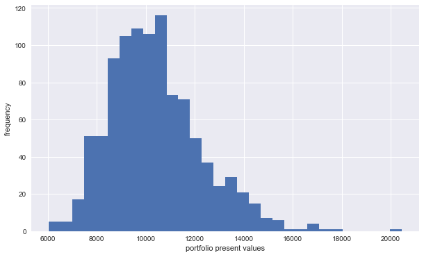
Some statistics via pandas.
[23]:
pdf = pd.DataFrame(pvs)
pdf.describe()
[23]:
| 0 | |
|---|---|
| count | 1000.000000 |
| mean | 10385.491824 |
| std | 1891.255451 |
| min | 6045.025829 |
| 25% | 9059.919260 |
| 50% | 10189.486685 |
| 75% | 11436.385373 |
| max | 20446.938649 |
The delta risk report.
[24]:
%%time
deltas, benchmark = port.get_port_risk(Greek='Delta', fixed_seed=True, step=0.2,
                                       risk_factors=list(risk_factors.keys())[:4])
risk_report(deltas)
  1_sv
0.8
1.0
1.2

  2_gbm
0.8
1.0
1.2

  3_gbm
0.8
1.0
1.2

  4_gbm
0.8
1.0
1.2


  1_sv_Delta
major  minor
0.8    factor       28.73
       value     10318.88
1.0    factor       35.91
       value     10385.48
1.2    factor       43.09
       value     10490.80
Name:   1_sv_Delta, dtype: float64

  2_gbm_Delta
major  minor
0.8    factor       30.36
       value     10410.14
1.0    factor       37.95
       value     10385.48
1.2    factor       45.54
       value     10391.22
Name:   2_gbm_Delta, dtype: float64

  3_gbm_Delta
major  minor
0.8    factor       30.04
       value     10440.04
1.0    factor       37.55
       value     10385.48
1.2    factor       45.06
       value     10421.06
Name:   3_gbm_Delta, dtype: float64

  4_gbm_Delta
major  minor
0.8    factor       22.29
       value     10429.74
1.0    factor       27.87
       value     10385.48
1.2    factor       33.44
       value     10351.02
Name:   4_gbm_Delta, dtype: float64
CPU times: user 5.2 s, sys: 502 ms, total: 5.71 s
Wall time: 4 s
The vega risk report.
[25]:
%%time
vegas, benchmark = port.get_port_risk(Greek='Vega', fixed_seed=True, step=0.2,
                                      risk_factors=list(risk_factors.keys())[:3])
risk_report(vegas)
  1_sv
0.8
1.0
1.2

  2_gbm
0.8
1.0
1.2

  3_gbm
0.8
1.0
1.2


  1_sv_Vega
major  minor
0.8    factor        0.42
       value     10377.30
1.0    factor        0.52
       value     10384.95
1.2    factor        0.62
       value     10402.19
Name:   1_sv_Vega, dtype: float64

  2_gbm_Vega
major  minor
0.8    factor        0.27
       value     10365.33
1.0    factor        0.34
       value     10384.95
1.2    factor        0.41
       value     10404.53
Name:   2_gbm_Vega, dtype: float64

  3_gbm_Vega
major  minor
0.8    factor        0.12
       value     10374.04
1.0    factor        0.14
       value     10384.95
1.2    factor        0.17
       value     10395.83
Name:   3_gbm_Vega, dtype: float64
CPU times: user 5.05 s, sys: 481 ms, total: 5.53 s
Wall time: 3.89 s
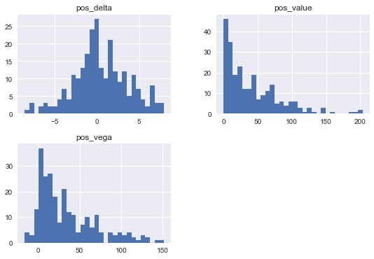
14.6. Visualization of Results
Selected results visualized.
[26]:
res[['pos_value', 'pos_delta', 'pos_vega']].hist(bins=30, figsize=(9, 6))
plt.ylabel('frequency')
[26]:
<matplotlib.text.Text at 0x111e61550>
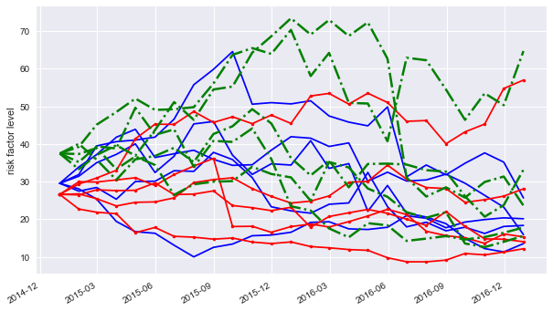
Sample paths for three underlyings.
[27]:
paths_0 = list(port.underlying_objects.values())[0]
paths_0.generate_paths()
paths_1 = list(port.underlying_objects.values())[1]
paths_1.generate_paths()
paths_2 = list(port.underlying_objects.values())[2]
paths_2.generate_paths()
[28]:
pa = 5
plt.figure(figsize=(10, 6))
plt.plot(port.time_grid, paths_0.instrument_values[:, :pa], 'b');
print('Paths for %s (blue)' % paths_0.name)
plt.plot(port.time_grid, paths_1.instrument_values[:, :pa], 'r.-');
print ('Paths for %s (red)' % paths_1.name)
plt.plot(port.time_grid, paths_2.instrument_values[:, :pa], 'g-.', lw=2.5);
print('Paths for %s (green)' % paths_2.name)
plt.ylabel('risk factor level')
plt.gcf().autofmt_xdate()
Paths for  48_sv (blue)
Paths for  12_jd (red)
Paths for  22_sv (green)
Copyright, License & Disclaimer
© Dr. Yves J. Hilpisch | The Python Quants GmbH
DX Analytics (the “dx library” or “dx package”) is licensed under the GNU Affero General Public License version 3 or later (see http://www.gnu.org/licenses/).
DX Analytics comes with no representations or warranties, to the extent permitted by applicable law.
http://tpq.io | dx@tpq.io | http://twitter.com/dyjh
Quant Platform | http://pqp.io
Python for Finance Training | http://training.tpq.io
Certificate in Computational Finance | http://compfinance.tpq.io
Derivatives Analytics with Python (Wiley Finance) | http://dawp.tpq.io
Python for Finance (2nd ed., O’Reilly) | http://py4fi.tpq.io